https://github.com/beastyblacksmith/moleculardynamics.jl

Julia utilities for reading in and analyzing Gromacs simulation results

https://github.com/beastyblacksmith/moleculardynamics.jl

Repository

Julia utilities for reading in and analyzing Gromacs simulation results

https://github.com/BeastyBlacksmith/MolecularDynamics.jl/blob/master/

MolecularDynamics
=================
James W. Barnett    
jbarnet4@tulane.edu

"MolecularDynamics" is a [Julia](http://www.julialang.org) package for the 
reading in and analysis of [Gromacs](http://www.gromacs.org) Molecular Dynamics
simulations. The goal is to provide a small and simple framework for simulation analysis.
This project does not intend to provide every analytical tool possible, but
instead intends to give a foundation for writing analysis software, making it
easier to work with Gromacs files in Julia. Several statistical packages are
available for Julia that can be used in conjunction with this package.

**NOTE**: This package is incompatible with Julia >= 0.6. I do not plan on
continuing to develop this package, but pull requests are welcome that update
the package to be compatible with 0.6 and above.

The following modules are included in this package:

*  Gmx - the main file processing module. Combines Xtc and Ndx functions to 
         be able to read in an xtc file into an
   array for processing.
*  Utils - the main analysis module.
*  Xtc - reads in xtc files.
*  Ndx - reads in ndx files.

Note that this is a work in progress and probably contains a few bugs. Please
check it out and give me some feedback.

Requirements
------------

The xdrfile library is required for reading in Gromacs xtc files. You can
[download it here](http://www.gromacs.org/Downloads) (bottom of the page). You
must enable building it as a shared library. Here is how to download and install
the library:

    wget ftp://ftp.gromacs.org/pub/contrib/xdrfile-1.1.1.tar.gz
    tar xvzf xdrfile-1.1.1.tar.gz
    cd xdrfile-1.1.1
    ./configure --enable-shared
    make -j N
    sudo make install

'N' is the number of processors with which to build.

Installation
------------

Open the REPL:

    julia

Now add the package:

    julia> Pkg.add("MolecularDynamics")

To start using the package do the following:

    julia> using MolecularDynamics

Example Usage
--------------

###Reading in files

Here are a few ways to use these modules in the REPL. Any of these functions can
be put into a script. Some examples are in the "examples" directory, including a
radial distribution calculation. 

The following uses "traj.xtc" and "index.ndx" from the "examples/gmx-test" 
directory, but you can use any xtc file and corresponding index file you wish. 
First open the REPL.

Now here are a few things you can do with "read_gmx". Read in an xtc file and
save all of the data to various variables:

    julia> g = read_gmx("traj.xtc"):

Your output should look something like this:

    First frame to save: 1
    Last frame to save: 100000
    Saving every frame.
    Initializing traj.xtc
    No. of atoms = 2014
    Saving all atoms.
    Saved 101 frames.

You can now access all of the saved information in the "g" object which has a type of
gmxType:

    juila> typeof(g)
    gmxType (constructor with 2 methods)

    julia> names(g)
    5-element Array{Symbol,1}:
     :no_frames
     :time     
     :box      
     :x        
     :natoms

How many frames were saved to "g". Note that Gromacs simulations start at time
0, which is saved to the first element in our arrays.

    julia> g.no_frames
    101

Time at a frame 5 (in ps):

    julia> g.time[5]
    0.8f0

The box at frame 10:

    julia> g.box[10]
    3/x3 Array{Float32,2}:
     2.45527  0.0      0.0    
     0.0      2.45527  0.0    
     0.0      0.0      2.45527

Coordinates of the 5th atom at frame 20. Note that we have a special dictionary
entry "all" since no index file was specified (see below when one is).

    julia> g.x["all"][20][:,5]
    3-element Array{Float32,1}:
     1.335
     1.142
     0.591

How many atoms are in "all":

    julia> g.natoms["all"]
    2014

We can also read in an index file and specify one or more index groups to be
saved. In this case we'll save the "C" and "CH2" groups:

    julia> g = read_gmx("traj.xtc","index.ndx","C","CH2"):
    First frame to save: 1
    Last frame to save: 100000
    Saving every frame.
    Initializing traj.xtc
    No. of atoms = 2014
    Saving the following index groups:
      C (4 elements)
      CH2 (6 elements)
    Saved 101 frames.

Time, box, and no_frames are the same as before. We can now access the
coordinates for each specific group. Here's the 2nd atom in the group "C" at the
10th frame. Note that we are using the key "C" now instead of "all". We could
also use "CH2" since we read that one in as well.

    julia> g.x["C"][10][:,2]
    3-element Array{Float32,1}:
     1.328
     1.141
     0.561

If you wanted just the x-coordinate of the above:

    julia> g.x["C"][10][1,2]
    1.3280001f0

Here is how many atoms are in the CH2 group:

    julia> g.natoms["CH2"]
    6

natoms and x are made up of dictionaries, as stated previously:

    julia> g.natoms
    Dict{Any,Any} with 2 entries:
      "CH2" => 6
      "C"   => 4

    julia> g.x
    Dict{Any,Any} with 2 entries:
      "CH2" => {
      "C"   => {

You can also save only specific frames to the gmxType object, specifying the first frame to save, the last frame to save, and whether or not to skip frames in saving. The following starts at the 5th frame and then ends at the 10th frame, saving only every other frame:

    julia> g = read_gmx("traj.xtc",5,10,2);
    First frame to save: 5
    Last frame to save: 10
    Saving every other frame.
    Initializing traj.xtc
    No. of atoms = 2014
    Saving all atoms.
    Saved 5 frames.

An index file can be specified with groups again:

    julia> g = read_gmx("traj.xtc",5,10,2,"index.ndx","C");
    First frame to save: 5
    Last frame to save: 10
    Saving every other frame.
    Initializing traj.xtc
    No. of atoms = 2014
    Saving the following index groups:
      C (4 elements)
    Saved 5 frames.

So far I've shown how to read in all the frames of an xtc file (or an index
group) and save them to a gmxType object. You can also read in the xtc file
frame-by-frame using the Xtc module:

First start initialize the file:

    juila> stat, xtc = xtc_init("traj.xtc")
    Initializing traj.xtc
    No. of atoms = 2014

    julia> stat
    0

    julia> typeof(xtc)
    xtcType (constructor with 1 method)

    juila> names(xtc)
    7-element Array{Symbol,1}:
     :natoms
     :step  
     :time  
     :box   
     :x     
     :prec  
     :xd   
    
"stat" is returned and tells if the initialization / read was successful (0 is success). "xd" is a C pointer that cannot be accessed from Julia and is solely used for getting the data using the C library xdrfile.

Now you can read the first frame using the xtc object above. 

    julia> stat, xtc = read_xtc(xtc)

Now you can get the info for the frame you just read in. Note that some of these
are zero element arrays for compatibility with the C library:

    julia> stat
    0

    julia> xtc.natoms
    2014

    juila> xtc.step[]
    0

    juila> xtc.time[]
    0.0f0

    juila> xtc.box
    3x3 Array{Float32,2}:
     2.47699  0.0      0.0    
     0.0      2.47699  0.0    
     0.0      0.0      2.47699

The coordinates of the first atom:

    juila> xtc.x[:,1]
    3-element Array{Float32,1}:
     1.297
     0.937
     0.483

They y-coordinate of the 3rd atom:

    juila> xtc.x[2,3]
    0.984f0

The precision:

    juila> xtc.prec[]
    1000.0f0
    
Note that the first read is at step 0 with a time of 0.0. That's just due to the way simulations work in Gromacs. Calling "read_xtc" again will read the next frame. Note that "read_xtc" returns a tuple with the first element giving the status of the read and the second giving an xtcType object containing all of the above information. You could simply place the "read_xtc" function in a loop and then do your calculations within the loop (the Gmx module does this but simply saves everything to a gmxType object). Once you're finished reading frames, you can close the xtc file:

    julia> stat = close_xtc(xtc)

    julia> stat
    0

You can also use the "read_ndx" module to probe the index file directly ("read_gmx"
does this when you specify an index file and index groups).

    julia> ndx = read_ndx("index.ndx");

"read_ndx" returns a dictionary containing all of the different index groups:

    juila> keys(ndx)
    KeyIterator for a Dict{Any,Any} with 8 entries. Keys:
    "Water"
    "System"
    "CH2"
    "CH3"
    "non-Water"
    "Other"
    "C"
    "SOL"

Specifying a key returns the locations of those atoms in the xtc file:

    julia> C_locations = ndx["C"]
    4-element Array{Int64,1}:
      1
      5
      8
     11

You could then access those atoms from an xtcType object:

    juila> import Xtc: xtc_init, read_xtc, close_xtc

    julia> stat, xtc = xtc_init("traj.xtc");
    Initializing traj.xtc
    No. of atoms = 2014

    juila> stat, xtc = read_xtc("traj.xtc")

These are the coordinates of just the "C" group from this frame:

    julia> xtc.x[:,C_locations]
    3x4 Array{Float32,2}:
     1.297  1.249  1.334  1.269
     0.937  1.021  1.145  1.21 
     0.483  0.601  0.638  0.762

As I stated earlier, some of these functions would be much more of use in a
script, so check out the examples.

###Analysis
Some basic functions are included in the Utils module. These include adjusting
for the periodic boundary condition (pbc), calculating bond angles
(bond_angle), and calculating dihedral angles (dih_angle).

####Periodic Boundary Condition
Use "pbc", Let's say you're interested in getting the distance between two atoms:

    julia> atom1 = g.x["C"][1][:,1]
    3-element Array{Float32,1}:
     0.443
     4.49 
     3.818

    julia> atom2 = g.x["OW"][1][:,1]
    3-element Array{Float32,1}:
     3.273
     0.392
     2.835

Here is the vector between these atoms:

    julia> a = atom1 - atom2
    3-element Array{Float32,1}:
     -2.83 
      4.098
      0.983

Now to adjust for the periodic boundary condition. Note I'm using the box from
the same frame as the coordinates above.

    julia> a = pbc(a,g.box[1])
    3-element Array{Float64,1}:
      2.1698  
     -0.901803
      0.983   

The magnitude is the distance:

    julia> sqrt(dot(a,a))
    2.547073301335343

####Bond Angles
Use "bond_angle". There are several different methods, all of which return
angles in radians:

Using the coordinate of three atoms that form an angle:

    julia> angle = bond_angle(g.x["C"][1][:,1],
                              g.x["C"][1][:,2],
                              g.x["C"][1][:,3],
                              g.box[1])
    2.082081985142061

Note that I'm just passing xyz coordinates as the first three arguments:

    julia> g.x["C"][1][:,1]
    3-element Array{Float32,1}:
     0.443
     4.49 
     3.818

Getting all the bond angles of an index group (like a linear alkane) for a
single frame - note the two different methods:

    julia> angle = bond_angle(g.x["C"][1],g.box[1])
    6-element Array{Float64,1}:
     2.08208
     1.93741
     2.01737
     1.87734
     2.02827
     2.01592

    julia> angle = bond_angle(g,"C",1)
    6-element Array{Float64,1}:
     2.08208
     1.93741
     2.01737
     1.87734
     2.02827
     2.01592

Getting all the angles of an index group for all frames (in this case octane
using only four frames - note there are two ways to do this):

    julia> angle = bond_angle(g.x["C"],g.box)
    6x4 Array{Float64,2}:
     2.08208  2.03211  1.96856  1.86377
     1.93741  1.92178  2.01451  1.92411
     2.01737  2.04895  1.93338  1.98445
     1.87734  1.98397  2.00395  1.8616 
     2.02827  2.00471  2.03594  2.04358
     2.01592  1.9744   1.83227  2.0012 

    julia> angle = bond_angle(g,"C")
    6x4 Array{Float64,2}:
     2.08208  2.03211  1.96856  1.86377
     1.93741  1.92178  2.01451  1.92411
     2.01737  2.04895  1.93338  1.98445
     1.87734  1.98397  2.00395  1.8616 
     2.02827  2.00471  2.03594  2.04358
     2.01592  1.9744   1.83227  2.0012 

And here is the first angle for all of the frames from this:

    julia> angle[1,:]
    1x4 Array{Float64,2}:
     2.08208  2.03211  1.96856  1.86377

Here are all of the angles for the first frame:

    julia> angle[:,1]
    6-element Array{Float64,1}:
     2.08208
     1.93741
     2.01737
     1.87734
     2.02827
     2.01592

####Dihedral Angles
Use the "dih_angle" function to calculate dihedral angles. There are several
methods. For now here are a few examples. Note that the dihedral angle is
returned in radians. 

Using the coordinates of four atoms making up the angle:

    julia> angle = dih_angle(g.x["C"][1][:,1],
                         g.x["C"][1][:,2],
                         g.x["C"][1][:,3],
                         g.x["C"][1][:,4],
                         g.box[1])
    -1.384181494375928

Using one frame to return all angles in a sequence (in this case all the angles
in octane - note the two different ways to do this):

    julia> g.x["C"][1]
    3x8 Array{Float32,2}:
     0.443  0.549  0.675  0.646  0.773  0.728  0.827  0.767
     4.49   4.461  4.547  4.685  4.775  4.891  4.929  0.017
     3.818  3.926  3.932  4.003  4.032  4.125  4.242  4.354

    julia> angle = dih_angle(g.x["C"][1], g.box[1])
    5-element Array{Float64,1}:
     -1.38418
     -3.00861
      2.95432
     -2.4199 
      2.8746 

    julia> angle = dih_angle(g,"C",1)
    5-element Array{Float64,1}:
     -1.38418
     -3.00861
      2.95432
     -2.4199 
      2.8746 

Using all frames to get all angles (in this case all frames of all carbons in octane;
I only read in the first four frames into "g" using "read_gmx"). Again, note the
two different ways of doing this:

    julia> angle = dih_angle(g.x["C"],g.box)
    5x4 Array{Float64,2}:
     -1.38418  -1.26239  -1.16925  -1.2465 
     -3.00861  -2.95298   3.00907  -2.70884
      2.95432   2.70807  -2.78729   3.09729
     -2.4199    2.92933   3.04705   2.89244
      2.8746    1.48004   1.14063   1.23341

    julia> angle = dih_angle(g,"C")
    5x4 Array{Float64,2}:
     -1.38418  -1.26239  -1.16925  -1.2465 
     -3.00861  -2.95298   3.00907  -2.70884
      2.95432   2.70807  -2.78729   3.09729
     -2.4199    2.92933   3.04705   2.89244
      2.8746    1.48004   1.14063   1.23341

The first angle in all frames:

    julia> angle[1,:]
    1x4 Array{Float64,2}:
     -1.38418  -1.26239  -1.16925  -1.2465

All angles in the first frame:

    julia> angle[:,1]
    5-element Array{Float64,1}:
     -1.38418
     -3.00861
      2.95432
     -2.4199 
      2.8746 

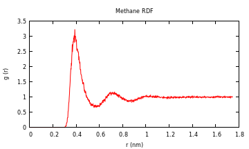
####Radial Distribution Function

First read in the two groups with "read_gmx". In this case it is the carbon of a
single methane and the water oxygens:

    julia> gmx = read_gmx(".julia/v0.3/MolecularDynamics/examples/rdf/traj.xtc",".julia/v0.3/MolecularDynamics/examples/rdf/index.ndx","C","OW");

Then pass the entire gmxType object and the name of the two groups to be used.
You'll receive a warning that this function is only for constant volume, cubic
box simulations at this point..

    julia> g = rdf(gmx,"C","OW");

Optionally you can select the binwidth (default: 0.002 nm) and the exclusion distance (default: 0.1 nm) for not
counting those atoms that are to close (and part of the same molecule):

    julia> g = rdf(gmx,"C","OW",0.002,0.1);

If you are just using one group (say you have several methanes and you want to
find the distribution between them), just pass one group name:

    julia> g = rdf(gmx,"C");

A tuple with the distances corresponding to the bins and the distribution is
returned. To plot quickly you can use the "Gaston" package:

    julia> using Gaston

    julia> plot(g[1],g[2],"title","","xlabel","r (nm)","ylabel","g(r)")

For the methane-methane radial distribution function from a simulation I did (10
methanes in water), the result looks like this:

!["Radial Distribution Function"](https://raw.githubusercontent.com/wesbarnett/MolecularDynamics.jl/master/images/rdf.png)

###Using Other Packages
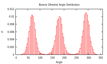
#### Dihedral Angle Distribution
As an example on how to use another package to help analyze some data, you could
use the Gaston package to plot a histogram of the dihedral angles of a molecule. For example, here is the distribution of butane
in water from a simulation I did at 293 K:

    julia> g = read_gmx("prd.xtc","index.ndx","C");
    First frame to save: 1
    Last frame to save: 100000
    Saving every frame.
    Initializing /home/james/testing/2_prd_313.xtc
    No. of atoms = 16494
    Saving the following index groups:
      C (4 elements)
    Saved 15001 frames.0

    julia> a = dih_angle(g.x["C"],g.box);

This just shifts everything below 0 to be from pi to 2pi:

    julia> a = map((x) -> if(x < 0.0) x += 2pi else x = x end, a);

Change from radians to degrees:

    julia> a = map((x) -> x * 180.0/pi, a);

Mean, median, and standard deviation of first angle (included in Standard
Library, so no need to add additional packages):

    julia> mean(a)
    182.7592278075726

    julia> median(a)
    181.339154595044

    julia> std(a)
    91.9910998654072

Install Gaston if you don't already have it:

    julia> Pkg.add("Gaston")

You'll also need gnuplot installed.
Now to plot the histogram:

    julia> using Gaston

    julia> histogram(a[1,:],"bins",360,"xlabel","Angle","ylabel","P","norm",1,"xrange","[0:360]","title","Dihedral Angle Distribution")

!["Dihedral angle
distribution"](https://raw.githubusercontent.com/wesbarnett/MolecularDynamics.jl/master/images/dih.png)

Contributing
------------

Please feel free to contribute to this project by forking the source code and then 
initiating pull requests. The development version of the project is in the branch "develop." Stable
versions of the project are in the branch "master" and tagged with release
numbers.

A few tests are done to see if a build is passing. Here is the develop branch
status:

!["status"](https://travis-ci.org/wesbarnett/MolecularDynamics.jl.svg?branch=develop)

Owner

GitHub Events