skytrackr

A tool to calculate geolocation by light positions using sky illuminance values (in lux). The routine uses model optimization and parameter estimation to determine locations robustly.

How to cite this package

You can cite this package like this "we obtained location estimates using the {skytrackr} R package (Hufkens 2023)". Here is the full bibliographic reference to include in your reference list (don't forget to update the 'last accessed' date):

Hufkens, K. (2023). skytrackr: a sky illuminance location tracker. Zenodo. https://doi.org/10.5281/zenodo.8331492.

Installation

development release

To install the development releases of the package run the following commands:

r if(!require(remotes)){install.packages("remotes")} remotes::install_github("bluegreen-labs/skytrackr") library("skytrackr")

Vignettes are not rendered by default, if you want to include additional documentation please use:

r if(!require(remotes)){install.packages("remotes")} remotes::install_github("bluegreen-labs/skytrackr", build_vignettes = TRUE) library("skytrackr")

Use

To demonstrate the functioning of the package a small demo dataset comprised of a couple of days of light logging of a Common swift near a nest box in Ghent, Belgium was included (i.e. tag cc876). I will use this data to demonstrate the features of the package. Note that when multiple dates are present all dates will be considered. The package is friendly to the use of R piped (|>) commands. Using all default settings you can just pipe the data in to the skytrackr() function. The returned object will be a data frame containing the best estimate (median) of the longitude and latitude as well as 5-95% quantile as sampled from the posterior parameter distribution.

Data pre-screening

During the breeding season it is advised to remove data which is affected by time spent on a nest, altering the light signal and position estimates. Both the light patterns and other sensory data can be used to restrict the data to migration and non-breeding movements.

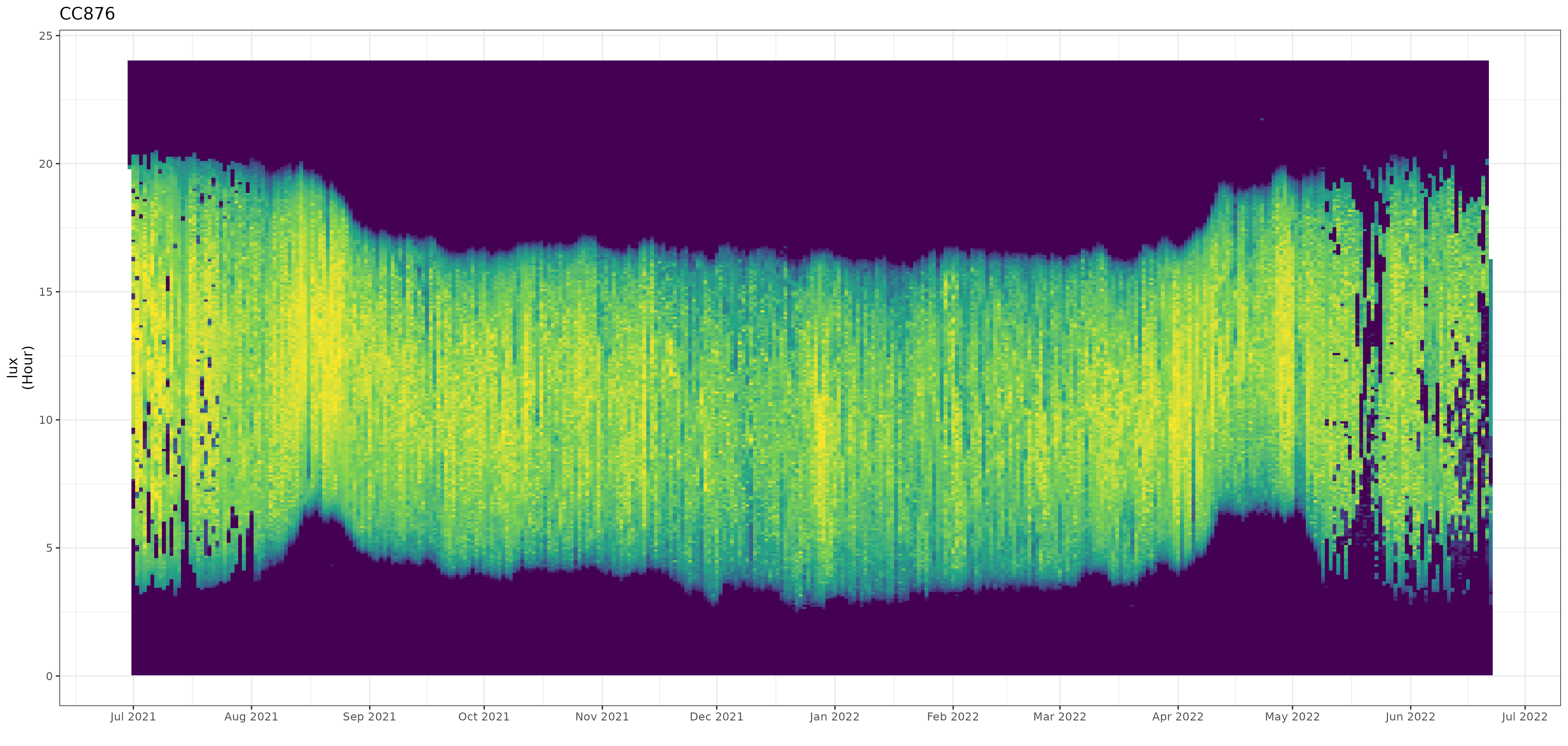
In the package I include the stk_profile() function which plots .lux files (and their ancillary .deg data) in an overview plot. The default plot is a static plot, however calling the function using the plotly = TRUE argument will render a dynamic plot on which you can zoom and which provides a tooltip showing the data values (including the date / time).

```r

read in the lux file, if a matching .deg

file is found it is integrated into one

long oriented data format

(here the internal demo data is used)

df <- stkreadlux( system.file("extdata/cc876.lux", package="skytrackr") )

plot the data as a static plot

stk_profile(df)

plot the data using plotly

(this allows exploring data values, e.g. zooming in and using a tooltip)

stk_profile(df, plotly = TRUE) ```

Date and time values of the non-breeding season can easily be determined and used in further sub-setting of the data for final processing. You can use the automated stk_screen_twl() function to remove dates with either stationary roosting behaviour (with dark values during daytime hours), or with "false" twilight events (due to birds roosting in dark conditions).

```r

filter data using twilight heuristics

and filter out the flagged values

df <- df |> stkscreentwl(filter = TRUE)

you can run the stk_profile() command again

to show the trimmed data, note all functions

are pipeable

df |> stk_profile() ```

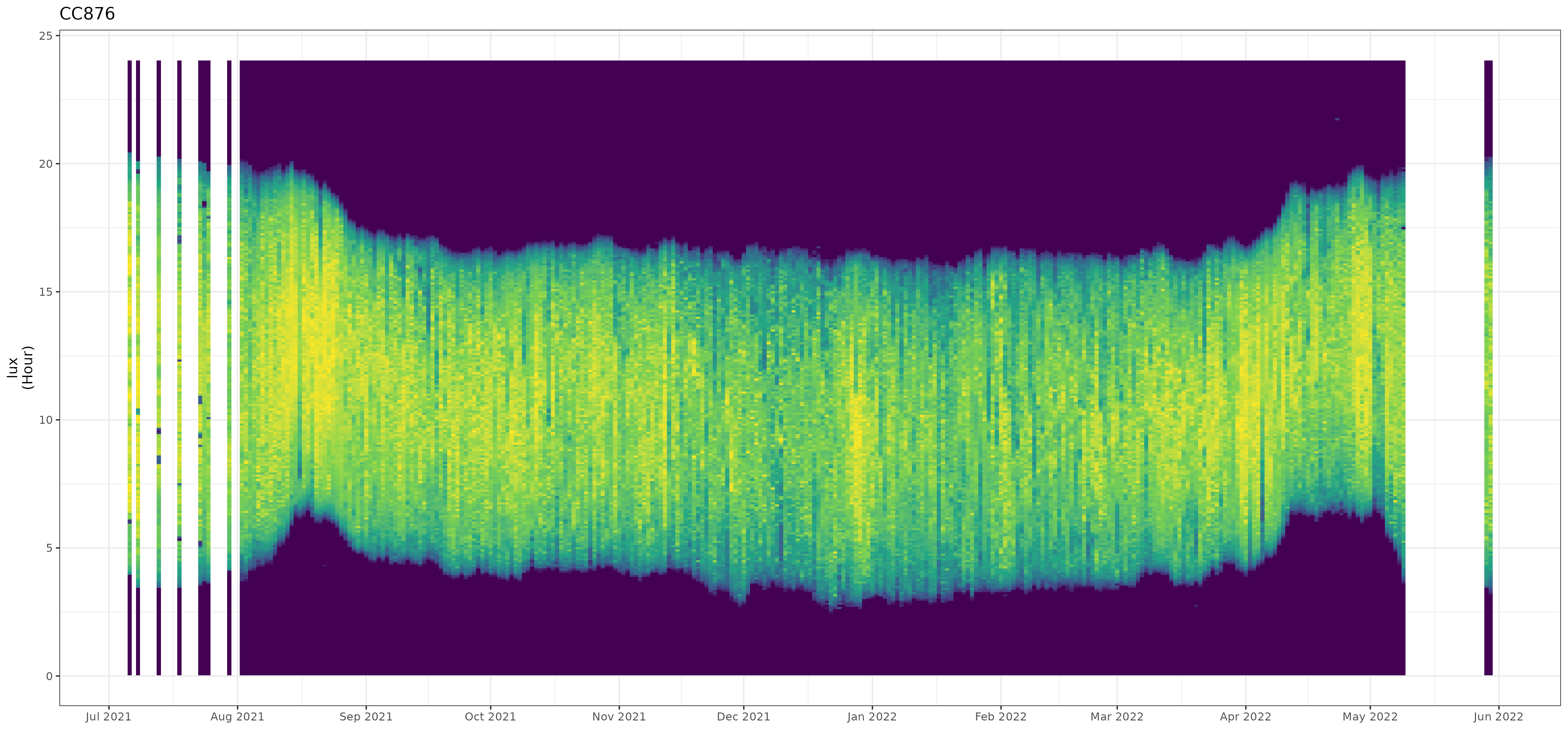
Further sub-setting can be done from this point, but if a bird is known to remain in a single location for breeding one can assume the individual is stationary. The filtering is there to provide as much of an hands off approach as possible, but use expert judgement.

MCMC DEzs optimization

To track movements by light using {skytrackr} you will need a few additional parameters. First, you will need to define the methodology used to find an optimal solution. The underlying BayesianTools package used in optimization allows for the specification of optimization techniques using the 'control' statement. The same argument can be used in the main skytrackr() routine.

In addition, care should be taken to specify the start location and tolerance (maximum degrees covered in a single flight - in km). The routine also needs you to specify an applicable land mask for land bound species. This land mask can be buffered extending somewhat offshore if desired. Finally, there is a behavioural component to the optimization routine used through the use of a step-selection function. This step-selection function determines the probability that a certain distance is covered based upon a probability density distribution provided by the user. Common distributions within movement ecology are for example a gamma or weibull distribution. Ideally these distributions are fit to previously collected data (either light-logger or GPS based), or based on common sense.

All three factors, the tolerance (maximum distance covered), the land mask (limiting locations to those over land), and step-selection function (providing a probabilistic constrained on distance covered), constrain the parameter fit. This ensures stability of results on a pseudo-mechanistic basis.

```r

define land mask with a bounding box

and an off-shore buffer (in km), in addition

you can specifiy the resolution of the resulting raster

mask <- stk_mask( bbox = c(-20, -40, 60, 60), #xmin, ymin, xmax, ymax buffer = 150, # in km resolution = 0.5 )

define a step selection distribution

ssf <- function(x, shape = 1.02, scale = 250, tolerance = 1500){ norm <- sum(stats::dgamma(1:tolerance, shape = shape, scale = scale)) prob <- stats::dgamma(x, shape = shape, scale = scale) / norm }

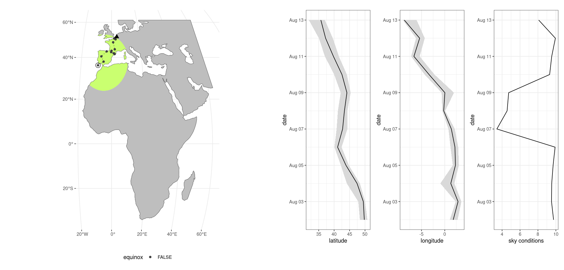
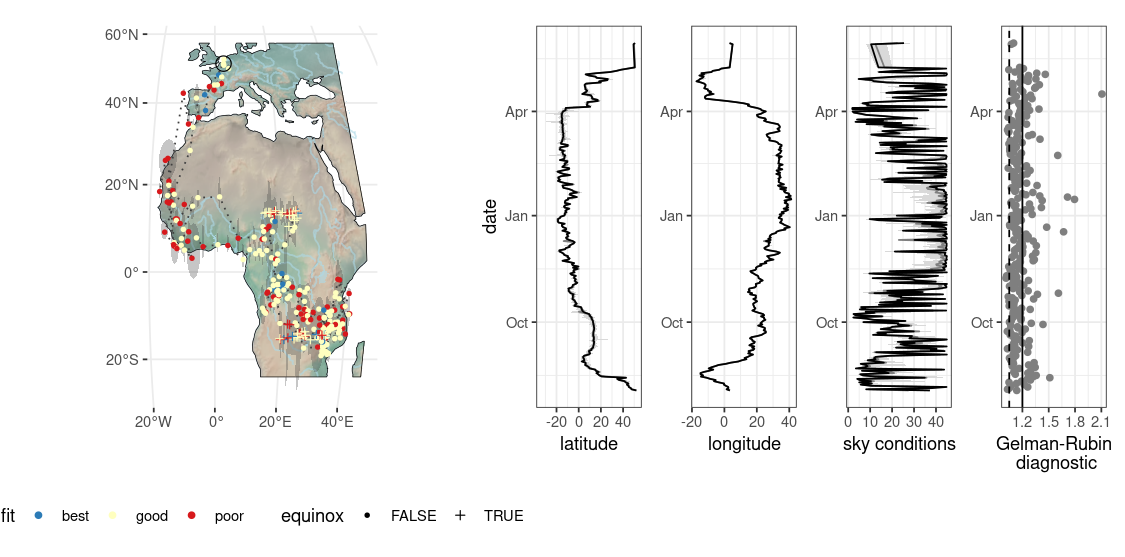
locations <- data |> skytrackr( startlocation = c(51.08, 3.73), tolerance = 1500, # in km scale = c(1,10), range = c(1.5, 140), control = list( sampler = 'DEzs', settings = list( burnin = 500, iterations = 1500, message = FALSE ) ), stepselection = ssf, mask = mask, plot = TRUE ) ```

If you enable plotting during the optimization routine a plot will be drawn with each new location which is determined. The plot shows a map covering the geographic extent as set by the mask you provide and a green region of interest defined by the intersection of the mask and a hard distance threshold tolerance (tolerance parameter). The start position is indicated with a black triangle, the latest position is defined by a closed and open circle combined.

During equinoxes the small closed circles will be small open circles as these periods have increased inherent uncertainty. To the right are also three panels showing the best value of the three estimated parameters as a black line, and their uncertainty intervals. Note that using the plotting option considerably slows down overall calculation due to rendering times (it is fun to watch though).

You can map the final location estimates using the same rendering layout using stk_map().

r locations |> stk_map(bbox = c(-20, -40, 60, 60))