https://github.com/ceyron/taylor-green-vortex-julia

A simple pseudo-spectral solver for the Direct Numerical Simulation (DNS) of the 3D Taylor-Green Vortex in the Julia programming language

https://github.com/ceyron/taylor-green-vortex-julia

Repository

A simple pseudo-spectral solver for the Direct Numerical Simulation (DNS) of the 3D Taylor-Green Vortex in the Julia programming language

https://github.com/Ceyron/taylor-green-vortex-julia/blob/main/

# 3D Taylor Green Vortex Simulation in Julia

![taylor_green_animation](https://user-images.githubusercontent.com/27728103/172134850-c7268c46-3443-4295-a937-ee44ca535a3c.gif)

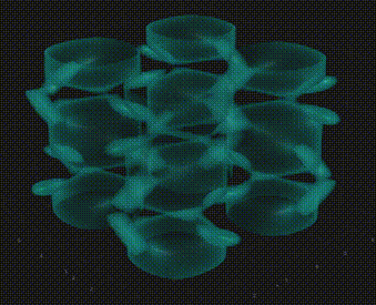
 Watch a [4K video of this](https://youtu.be/7dDAlm35ftM).

 A pseudo-spectral solver for the 3D Taylor-Green Vortex using the Fast Fourier Transformation (FFT) . The implemenation is based on the [Spectral DNS in Python Repo](https://github.com/spectralDNS/spectralDNS).

The 3D Taylor Green Vortex is a common test case for Direct Numerical Simulation of Turbulence. Due to its 3D periodic domain it is a perfect candidate for a pseudo-spectral solver that allows for fine discretizations at manageable computational cost (due to the *N log(N)* scaling properties of the FFT) .

You can [watch a code-along implementation](https://youtu.be/QNJeWgVLML8) here.

The Taylor Green Vortex builds upon the (incompressible) Navier-Stokes equations:


    u/t + (u  ) u =  1/ p +  u + f
      u = 0

The domain is:

     = (0, 2)

For the Taylor-Green Vortex we have the following simplifications:

     = 1
    f = 0

The kinematic viscosity is set to:

     = 1/1600

The crucial incredient to the Taylor Green Vortex is the initial condition:

    u(t=0, x, y, z) =   sin(x)cos(y)cos(z)
    v(t=0, x, y, z) =  cos(x)sin(y)cos(z)
    w(t=0, x, y, z) = 0

This initial state results in many stages all the way to full turbulence and, finally, a dissipation and decay.

---

 Also check out the [Repo](https://github.com/Ceyron/machine-learning-and-simulation) of my [YouTube Channel](https://www.youtube.com/c/MachineLearningSimulation) for similar simple simulation scripts in Julia and Python.

---

The solution strategy in the file is based on [this paper by Mortensen & Langtangen](https://arxiv.org/abs/1602.03638).

Let's make the following definitions

    u  : The velocity field (3D vector) in spatial domain
      : The velocity field (3D vector) in Fourier domain

      : The vorticity field (3D vector) in spatial domain
      : The vorticity field (3D vector) in Fourier domain

    m  : The product of vorticity and velocity (3D vector) in spatial domain
      : The product of vorticity and velocity (3D vector) in Fourier domain

    k  : The wavenumber vector (3D vector)

      : The pressure in Fourier domain (1D scalar)

    b  : The rhs of the ODE system in Fourier domain (3D vector)

    i  : The imaginary unit (1D scalar)

0. Initialize the velocity vectors according to the IC and transform them into
   Fourier Domain
1. Compute the curl in Fourier Domain by means of a cross
   product with the wavenumber vector and imaginary unit

         = () = (  u) = i k  

2. Transform the vorticity back to spatial domain

         = ()

3. Compute the "convection" by means of a cross product

        m = u  

4. Transform the "convection" back into Fourier domain

         = (m)

5. Perform a dealising on the convection in order to suppress unresolved wave numbers

6. Compute the (pseudo) "pressure" in Fourier domain

         = (k  ) / ||k||

7. Compute the rhs to the ODE system

        b = m -  ||k||  - (k ) / ||k||

8. Advance the velocity in Fourier Domain by means of an
   Explicit Euler time step
   
           + t b

9. Transform the newly obtained velocity back into spatial 
   domain

        u = ()

10. (Optional) visualize the vorticity magnitude in spatial
   domain interactively

11. Repeat from (1.)


In total, it takes us three (three-dimensional) Fourier Transforms per time
iteration:

- Transformation of the curl to spatial domain
- Transformation of the "convection" to Fourier Domain
- Transformation of the velocity to spatial domain

It is called pseudo-spectral because some operations are performed in Fourier
Domain and some in the spatial domain.

Owner

GitHub Events