kalepy
kalepy: a Python package for kernel density estimation, sampling and plotting - Published in JOSS (2021)
Science Score: 95.0%
This score indicates how likely this project is to be science-related based on various indicators:
-
○CITATION.cff file
-
✓codemeta.json file
Found codemeta.json file -
✓.zenodo.json file
Found .zenodo.json file -
✓DOI references
Found 5 DOI reference(s) in README and JOSS metadata -
✓Academic publication links
Links to: joss.theoj.org, zenodo.org -
✓Committers with academic emails
1 of 4 committers (25.0%) from academic institutions -
○Institutional organization owner
-
✓JOSS paper metadata
Published in Journal of Open Source Software
Keywords
Repository
Kernel Density Estimation and (re)sampling
Basic Info
Statistics
- Stars: 62
- Watchers: 5
- Forks: 12
- Open Issues: 14
- Releases: 2
Topics
Metadata Files
README.md
kalepy: Kernel Density Estimation and Sampling
![]()
![]()

![]()
![]()
This package performs KDE operations on multidimensional data to: 1) calculate estimated PDFs (probability distribution functions), and 2) resample new data from those PDFs.
Documentation
A number of examples (also used for continuous integration testing) are included in the package notebooks. Some background information and references are included in the JOSS paper.
Full documentation is available on kalepy.readthedocs.io.
README Contents
Installation
from pypi (i.e. via pip)
bash
pip install kalepy
from source (e.g. for development)
bash
git clone https://github.com/lzkelley/kalepy.git
pip install -e kalepy/
In this case the package can easily be updated by changing into the source directory, pulling, and rebuilding:
```bash cd kalepy git pull pip install -e .
Optional: run unit tests (using the pytest package)
pytest ```
Basic Usage
```python import numpy as np import matplotlib.pyplot as plt import matplotlib as mpl
import kalepy as kale
from kalepy.plot import nbshow ```
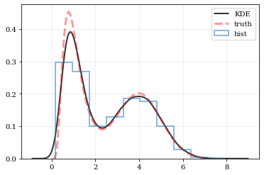
Generate some random data, and its corresponding distribution function
```python NUM = int(1e4) np.random.seed(12345)
Combine data from two different PDFs
d1 = np.random.normal(4.0, 1.0, NUM) _d2 = np.random.lognormal(0, 0.5, size=NUM) data = np.concatenate([d1, _d2])
Calculate the "true" distribution
xx = np.linspace(0.0, 7.0, 100)[1:] yy = 0.5np.exp(-(xx - 4.0)2/2) / np.sqrt(2np.pi) yy += 0.5 * np.exp(-np.log(xx)2/(2*0.52)) / (0.5xxnp.sqrt(2*np.pi)) ```
Plotting Smooth Distributions
```python
Reconstruct the probability-density based on the given data points.
points, density = kale.density(data, probability=True)
Plot the PDF
plt.plot(points, density, 'k-', lw=2.0, alpha=0.8, label='KDE')
Plot the "true" PDF
plt.plot(xx, yy, 'r--', alpha=0.4, lw=3.0, label='truth')
Plot the standard, histogram density estimate
plt.hist(data, density=True, histtype='step', lw=2.0, alpha=0.5, label='hist')
plt.legend() nbshow() ```
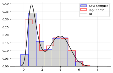
resampling: constructing statistically similar values
Draw a new sample of data-points from the KDE PDF
```python
Draw new samples from the KDE reconstructed PDF
samples = kale.resample(data)
Plot new samples
plt.hist(samples, density=True, label='new samples', alpha=0.5, color='0.65', edgecolor='b')
Plot the old samples
plt.hist(data, density=True, histtype='step', lw=2.0, alpha=0.5, color='r', label='input data')
Plot the KDE reconstructed PDF
plt.plot(points, density, 'k-', lw=2.0, alpha=0.8, label='KDE')
plt.legend() nbshow() ```
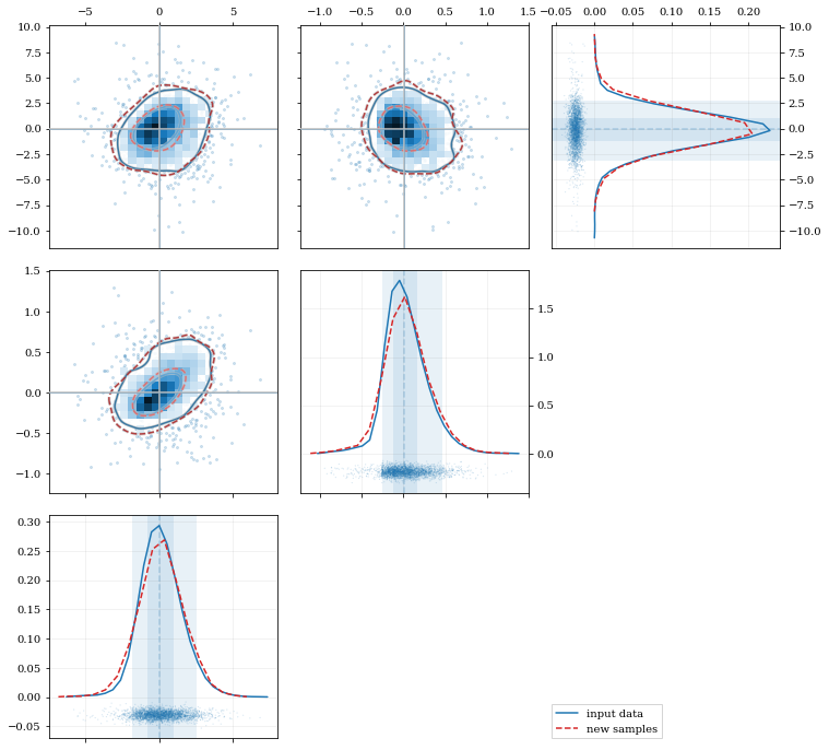
Multivariate Distributions
```python reload(kale.plot)
Load some random-ish three-dimensional data
np.random.seed(9485) data = kale.utils.randomdata3d02(num=3e3)
Construct a KDE
kde = kale.KDE(data)
Construct new data by resampling from the KDE
resamp = kde.resample(size=1e3)
Plot the data and distributions using the builtin kalepy.corner plot
corner, h1 = kale.corner(kde, quantiles=[0.5, 0.9]) h2 = corner.clean(resamp, quantiles=[0.5, 0.9], dist2d=dict(median=False), ls='--')
corner.legend([h1, h2], ['input data', 'new samples'])
nbshow() ```
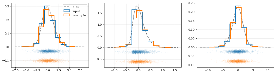
```python
Resample the data (default output is the same size as the input data)
samples = kde.resample()
---- Plot the input data compared to the resampled data ----
fig, axes = plt.subplots(figsize=[16, 4], ncols=kde.ndim)
for ii, ax in enumerate(axes):
# Calculate and plot PDF for iith parameter (i.e. data dimension ii)
xx, yy = kde.density(params=ii, probability=True)
ax.plot(xx, yy, 'k--', label='KDE', lw=2.0, alpha=0.5)
# Draw histograms of original and newly resampled datasets
*, h1 = ax.hist(data[ii], histtype='step', density=True, lw=2.0, label='input')
*, h2 = ax.hist(samples[ii], histtype='step', density=True, lw=2.0, label='resample')
# Add 'kalepy.carpet' plots showing the data points themselves
kale.carpet(data[ii], ax=ax, color=h1[0].getfacecolor())
kale.carpet(samples[ii], ax=ax, color=h2[0].getfacecolor(), shift=ax.get_ylim()[0])
axes[0].legend() nbshow() ```
Fancy Usage
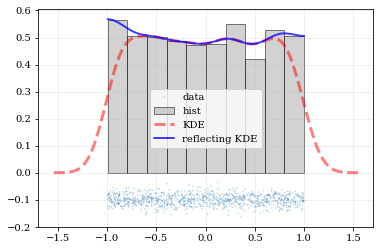
Reflecting Boundaries
What if the distributions you're trying to capture have edges in them, like in a uniform distribution between two bounds? Here, the KDE chooses 'reflection' locations based on the extrema of the given data.
```python
Uniform data (edges at -1 and +1)
NDATA = 1e3 np.random.seed(54321) data = np.random.uniform(-1.0, 1.0, int(NDATA))
Create a 'carpet' plot of the data
kale.carpet(data, label='data')
Histogram the data
plt.hist(data, density=True, alpha=0.5, label='hist', color='0.65', edgecolor='k')
---- Standard KDE will undershoot just-inside the edges and overshoot outside edges
points, pdfbasic = kale.density(data, probability=True) plt.plot(points, pdfbasic, 'r--', lw=3.0, alpha=0.5, label='KDE')
---- Reflecting KDE keeps probability within the given bounds
setting reflect=True lets the KDE guess the edge locations based on the data extrema
points, pdfreflect = kale.density(data, reflect=True, probability=True) plt.plot(points, pdfreflect, 'b-', lw=2.0, alpha=0.75, label='reflecting KDE')
plt.legend() nbshow() ```
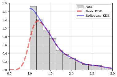
Explicit reflection locations can also be provided (in any number of dimensions).
```python
Construct random data, add an artificial 'edge'
np.random.seed(5142) edge = 1.0 data = np.random.lognormal(sigma=0.5, size=int(3e3)) data = data[data >= edge]
Histogram the data, use fixed bin-positions
edges = np.linspace(edge, 4, 20) plt.hist(data, bins=edges, density=True, alpha=0.5, label='data', color='0.65', edgecolor='k')
Standard KDE with over & under estimates
points, pdfbasic = kale.density(data, probability=True) plt.plot(points, pdfbasic, 'r--', lw=4.0, alpha=0.5, label='Basic KDE')
Reflecting KDE setting the lower-boundary to the known value
There is no upper-boundary when None is given.
points, pdfbasic = kale.density(data, reflect=[edge, None], probability=True) plt.plot(points, pdfbasic, 'b-', lw=3.0, alpha=0.5, label='Reflecting KDE')
plt.gca().set_xlim(edge - 0.5, 3) plt.legend() nbshow() ```
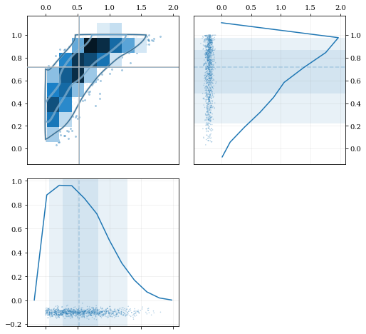
Multivariate Reflection
```python
Load a predefined dataset that has boundaries at:
x: 0.0 on the low-end
y: 1.0 on the high-end
data = kale.utils.randomdata2d03()
Construct a KDE with the given reflection boundaries given explicitly
kde = kale.KDE(data, reflect=[[0, None], [None, 1]])
Plot using default settings
kale.corner(kde)
nbshow() ```
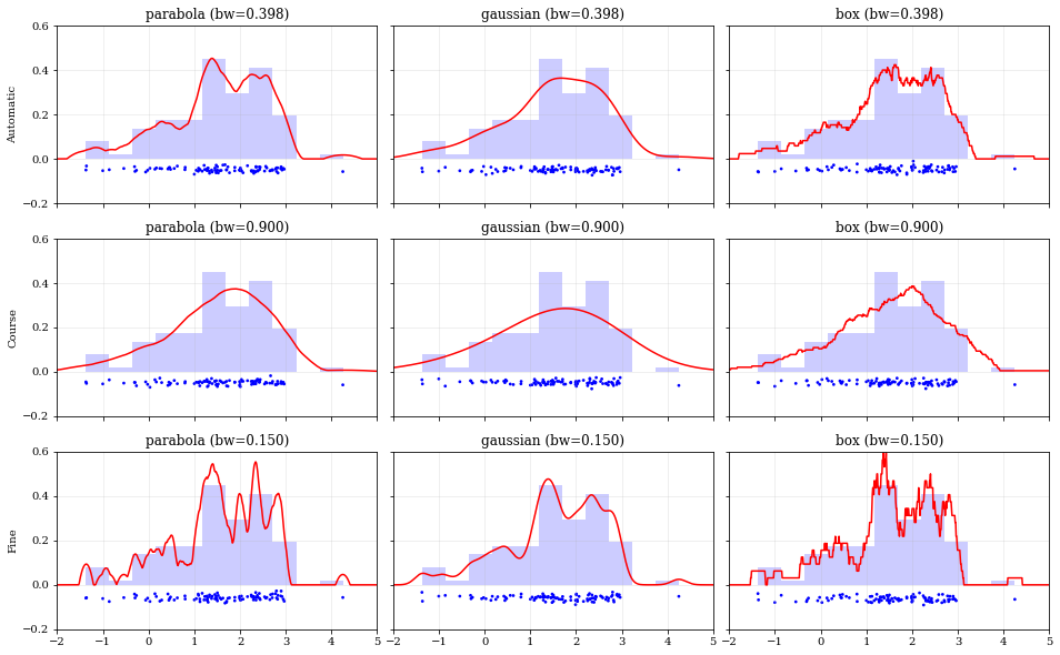
Specifying Bandwidths and Kernel Functions
```python
Load predefined 'random' data
data = kale.utils.randomdata1d02(num=100)
Choose a uniform x-spacing for drawing PDFs
xx = np.linspace(-2, 8, 1000)
------ Choose the kernel-functions and bandwidths to test -------
kernels = ['parabola', 'gaussian', 'box'] #
bandwidths = [None, 0.9, 0.15] # None means let kalepy choose #
-----------------------------------------------------------------
ylabels = ['Automatic', 'Course', 'Fine'] fig, axes = plt.subplots(figsize=[16, 10], ncols=len(kernels), nrows=len(bandwidths), sharex=True, sharey=True) plt.subplots_adjust(hspace=0.2, wspace=0.05) for (ii, jj), ax in np.ndenumerate(axes):
# ---- Construct KDE using particular kernel-function and bandwidth ---- #
kern = kernels[jj]                                                       #
bw = bandwidths[ii]                                                      #
kde = kale.KDE(data, kernel=kern, bandwidth=bw)                          #
# ---------------------------------------------------------------------- #

# If bandwidth was set to `None`, then the KDE will choose the 'optimal' value
if bw is None:
    bw = kde.bandwidth[0, 0]

ax.set_title('{} (bw={:.3f})'.format(kern, bw))
if jj == 0:
    ax.set_ylabel(ylabels[ii])

# plot the KDE
ax.plot(*kde.pdf(points=xx), color='r')
# plot histogram of the data (same for all panels)
ax.hist(data, bins='auto', color='b', alpha=0.2, density=True)
# plot  carpet   of the data (same for all panels)
kale.carpet(data, ax=ax, color='b')
ax.set(xlim=[-2, 5], ylim=[-0.2, 0.6]) nbshow() ```
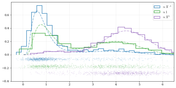
Resampling
Using different data weights
```python
Load some random data (and the 'true' PDF, for comparison)
data, truth = kale.utils.randomdata1d01()
---- Resample the same data, using different weightings ----
resampuni = kale.resample(data, size=1000) # resampsqr = kale.resample(data, weights=data2, size=1000) # resamp_inv = kale.resample(data, weights=data-1, size=1000) #
------------------------------------------------------------ #
---- Plot different distributions ----
Setup plotting parameters
kw = dict(density=True, histtype='step', lw=2.0, alpha=0.75, bins='auto')
xx, yy = truth samples = [resampinv, resampuni, resamp_sqr] yvals = [yy/xx, yy, yyxx*2/10] labels = [r'$\propto X^{-1}$', r'$\propto 1$', r'$\propto X^2$']
plt.figure(figsize=[10, 5])
for ii, (res, yy, lab) in enumerate(zip(samples, yvals, labels)): hh, = plt.plot(xx, yy, ls='--', alpha=0.5, lw=2.0) col = hh.get_color() kale.carpet(res, color=col, shift=-0.1ii) plt.hist(res, color=col, label=lab, *kw)
plt.gca().set(xlim=[-0.5, 6.5])
Add legend
plt.legend()
display the figure if this is a notebook
nbshow() ```
Resampling while 'keeping' certain parameters/dimensions
```python
Construct covariant 2D dataset where the 0th parameter takes on discrete values
xx = np.random.randint(2, 7, 1000) yy = np.random.normal(4, 2, xx.size) + xx**(3/2) data = [xx, yy]
2D plotting settings: disable the 2D histogram & disable masking of dense scatter-points
dist2d = dict(hist=False, mask_dense=False)
Draw a corner plot
kale.corner(data, dist2d=dist2d)
nbshow() ```
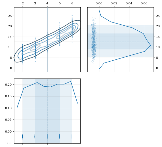
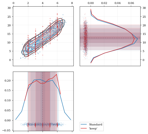
A standard KDE resampling will smooth out the discrete variables, creating a smooth(er) distribution. Using the keep parameter, we can choose to resample from the actual data values of that parameter instead of resampling with 'smoothing' based on the KDE.
```python kde = kale.KDE(data)
---- Resample the data both normally, and 'keep'ing the 0th parameter values ----
resampstnd = kde.resample() # resampkeep = kde.resample(keep=0) #
---------------------------------------------------------------------------------
corner = kale.Corner(2) dist2d['median'] = False # disable median 'cross-hairs' h1 = corner.plot(resampstnd, dist2d=dist2d) h2 = corner.plot(resampkeep, dist2d=dist2d)
corner.legend([h1, h2], ['Standard', "'keep'"]) nbshow() ```
Development & Contributions
Please visit the github page <https://github.com/lzkelley/kalepy>_ for issues or bug reports. Contributions and feedback are very welcome.
Contributors: * Luke Zoltan Kelley (@lzkelley) * Zachary Hafen (@zhafen)
JOSS Paper: * Kexin Rong (@kexinrong) * Arfon Smith (@arfon) * Will Handley (@williamjameshandley)
Attribution
A JOSS paper has been submitted. If you have found this package useful in your research, please add a reference to the code paper:
.. code-block:: tex
@article{kalepy,
  author = {Luke Zoltan Kelley},
  title = {kalepy: a python package for kernel density estimation and sampling},
  journal = {The Journal of Open Source Software},
  publisher = {The Open Journal},
}
Owner
- Name: Luke Zoltan Kelley
- Login: lzkelley
- Kind: user
- Location: Berkeley, CA
- Website: www.lzkelley.com
- Repositories: 23
- Profile: https://github.com/lzkelley
Theoretical astrophysics at the interface of gravitational waves, transients and cosmological environments.
JOSS Publication
kalepy: a Python package for kernel density estimation, sampling and plotting
Authors

Center for Interdisciplinary Exploration and Research in Astrophysics (CIERA), Northwestern University, USA, Physics & Astronomy, Northwestern University, USA
Editor
Arfon Smith
Tags
astronomy statistics monte carlo methodsGitHub Events
Total
- Issues event: 2
- Watch event: 6
Last Year
- Issues event: 2
- Watch event: 6
Committers
Last synced: 11 months ago
Top Committers
| Name | Commits | |
|---|---|---|
| lzkelley | l****y@g****m | 406 |
| lzkelley | l****y@c****u | 202 |
| Zachary Hafen | z****n@g****m | 4 |
| Arfon Smith | a****n | 2 |
Committer Domains (Top 20 + Academic)
Issues and Pull Requests
Last synced: 10 months ago
All Time
- Total issues: 15
- Total pull requests: 4
- Average time to close issues: 2 months
- Average time to close pull requests: 6 days
- Total issue authors: 8
- Total pull request authors: 4
- Average comments per issue: 0.73
- Average comments per pull request: 0.5
- Merged pull requests: 3
- Bot issues: 0
- Bot pull requests: 0
Past Year
- Issues: 1
- Pull requests: 0
- Average time to close issues: N/A
- Average time to close pull requests: N/A
- Issue authors: 1
- Pull request authors: 0
- Average comments per issue: 0.0
- Average comments per pull request: 0
- Merged pull requests: 0
- Bot issues: 0
- Bot pull requests: 0
Top Authors
Issue Authors
- lzkelley (8)
- jonathanoostvogels (1)
- arbenede (1)
- myradio (1)
- Pablobala (1)
- matthewkenzie (1)
- mx-eff (1)
- jbergner (1)
Pull Request Authors
- lzkelley (1)
- arfon (1)
- zhafen (1)
- apereiroc (1)
Top Labels
Issue Labels
Pull Request Labels
Packages
- Total packages: 1
-
Total downloads:
- pypi 583 last-month
- Total dependent packages: 3
- Total dependent repositories: 3
- Total versions: 18
- Total maintainers: 1
pypi.org: kalepy
Kernel Density Estimation (KDE) and sampling.
- Homepage: https://github.com/lzkelley/kalepy/
- Documentation: https://kalepy.readthedocs.io/
- License: MIT
-
Latest release: 1.4.3
published about 3 years ago
Rankings
Maintainers (1)
Dependencies
- actions/checkout v3 composite
- actions/setup-python v3 composite
- pypa/gh-action-pypi-publish master composite
- ipykernel *
- nbsphinx *
- flake8 * development
- gitpython * development
- jupyter * development
- nbconvert * development
- pytest * development
- sphinx_rtd_theme * development
- tox * development
- matplotlib >=3
- numba *
- numpy *
- scipy *
- six *
- actions/checkout v2 composite
- actions/setup-python v2 composite
- codecov/codecov-action v3 composite
- actions/checkout v3 composite
- actions/setup-python v3 composite