Discovering Themes in Text with Topic Modeling (Latent Dirichlet Allocation)

Description

The method uncovers hidden themes as semantic structures that are frequently discussed in the documents to explore unfamiliar domains. It may also be used to identify features as topics for subsequent tasks. For example, applying the method to the hotel reviews corpus may result in topics that represent food quality, menu, table service, pricing, and so on. It calculates the co-occurrence frequencies among words to organize topics as ordered collections of words and documents as ordered collections of topics. As an unsupervised approach, the topics are unlabeled and are represented by their most probable words. The method reads input as a document per line and outputs two files: document-topic distribution and topic-word distribution.

Use Cases

To explore the main topics discussed in political poll reviews of different user groups and analyze how the topics vary across these groups. The topics may include health care, immigration, the economy, etc., and are represented through their most prominent words.

Input Data

The input can be any text to explore. For demonstration purposes, we use BBC news article headlines as sample documents. Below are 10 example headlines taken from the dataset, which can be found in the file data/input-data/news-headings.txt

| Headlines | |--------------------------| | India calls for fair trade rules | | Sluggish economy hits German jobs | | Indonesians face fuel price rise | | Court rejects $280bn tobacco case | | Dollar gains on Greenspan speech | | Mixed signals from French economy | | Ask Jeeves tips online ad revival | | Rank 'set to sell off film unit' | | US trade gap hits record in 2004 | | India widens access to telecoms | |...|

Output Data

The latent topics identified are represented by the most significant words and their probabilities. It is similar to clustering in the sense that the words are grouped as topics and labeled un-intuitively as topic 1, topic 2, etc. However, unlike clustering, the words have probabilities of relevance to the topic.

Topic-word distribution: Topic word distribution provides the top few words for each topic with their probabilities, organized in decreasing order of their probabilities, indicating relevance to the topic.

The following are 3 topics (numTopics=3 in config.json) from the sample data, each with its top 10 words (wordsPerTopic=10 in config.json) and their probabilities.

| | Topic 1 | Topic 2 | Topic 3 | |---------|---------|---------|---------| | w1 | (new, 0.0158) |(win, 0.009) | (film, 0.0123) | | w2 | (Blair, 0.0136)| (deal, 0.0087) | (set, 0.0089) | | w3 | (hits, 0.0096) | (show, 0.0087) | (top, 0.008) | | w4 | (net, 0.009) | (shares, 0.0068) | (hit, 0.0077) | | w5 | (election, 0.0071)| (plan, 0.0068) | (wins, 0.0074) | | w6 | (Labour, 0.0071)| (firm, 0.0065) | (return, 0.0071) | | w7 | (growth, 0.0065)| (China, 0.0065) | (bid, 0.0071) | | w8 | (face, 0.0062) |( back, 0.0065) | (gets, 0.0065) | | w9 | (says, 0.0062) | (takes, 0.0065) | (Brown, 0.0065) | | w10 | (row, 0.0062) | (Yukos, 0.0062) | (economy, 0.0061) |

The complete distribution is written to data/output-data/topic-word-distribution.tsv

Document-topic distribution: Each document is assigned probabilities of representing a topic based on the topic association of its words. These probabilities indicate the extent to which the topics are discussed in these documents. For example, document 1 can be 37.5% topic 1, 25% topic 2, and 37.5% topic 3.

In case a reader is interested in only reading more about topic 1, he/she may only focus on the documents where topic 1 is the major topic.

| |Topic 1 | Topic 2 | Topic 3 | Text | |-----------|------------|----------|----------|---------------------| | Doc 1 | 0.3750 | 0.2500 | 0.3750 | India calls for fair trade rules | | Doc 2 | 0.3750 | 0.2500 | 0.3750 | Sluggish economy hits German jobs | | Doc 3 | 0.3750 | 0.2500 | 0.3750 | Indonesians face fuel price rise | | Doc 4 | 0.3750 | 0.3750 | 0.2500 | Court rejects $280bn tobacco case | | Doc 5 | 0.1429 | 0.2857 | 0.5714 | Dollar gains on Greenspan speech | | ... |

Written in file data/output-data/document-topic-distribution.tsv

Hardware Requirements

The method runs on a small virtual machine provided by a cloud computing company (2 x86 CPU core, 4 GB RAM, 40GB HDD).

Environment setup

To set up the working environment, execute the command

pip install -r requirements.txt

How to Use

• Execute notebook cells `LDA-collapsed-gibbs-sampling.ipynb to reproduce the sample results using sample input data and configurations.

• Copy your data to data/input-data/news-headings.txt, having a document (text unit) per line.

• To execute the method under different configurations, modify the settings in config.json. Specifics on configuration parameters and their values are provided in LDA-collapsed-gibbs-sampling.ipynb Section A.2

Technical Details

This method represents the Latent Dirichlet Allocation (LDA) topic modeling approach. It uses collapsed Gibbs sampling (LDA with collapsed Gibbs sampling) as the inference technique, which is an efficient extension of Gibbs sampling. The inference technique decides the most suitable topic for the sampled word, given the current state of the model, where the state of the model is determined by its document-topic distribution (having probabilities of each topic in each document) and topic-word distribution (having probabilities of each word in each topic). When a word switches its topic, i.e., its most suitable topic in the current state is different from its present topic (assigned in the previous iteration), it results in changing the state of the model. In each iteration, the inference technique samples each word to estimate its most suitable topic given the current state of the model. At the end of the iteration, the document-topic and topic-word probabilities are recomputed, and the model's state is updated.

The model starts with random initialization, i.e., the words are assigned to topics at random to help generate the initial probabilities for representing the initial state of the model. In the initial iterations, the word switch their topics more rigorously, which reduces in the subsequent iterations as more and more words settle in their respective topics. Using the Markov chain Monte Carlo (MCMC) approach, the next state of the model is determined from the current state of the model, converging on a stable distribution. Allowing collapsed Gibbs sampling with enough iterations (in a few thousand), the words are expected to settle down in their respective topics. Although starting from any random state, the model converges to similar probability distributions; however, a better initial state helps to converge in fewer iterations. As an unsupervised method, the topics are not labeled but rather represented by their highest probability (top presentable) words. Each topic is an ordered list of words, where the words are organized by their probabilities with the topic (calculated based on the co-occurrence frequency of the word with all the other words in the topic) in decreasing order.

The method has two hyperparameters, i.e., $\alpha$ as the Dirichlet prior for the document-topic distribution and $\beta$ as the Dirichlet prior for the topic-word distribution. This implementation uses the optimum values advised for the method. These Dirichlet priors control the bias or variance in the model's distribution. For example, when the $\alpha$ value is 1, the document-topic distribution is fully drawn from the input data without the prior affecting it. However, when its value is higher (generally in multiples of 10 as 100, 1000, ...), it introduces bias into the model. The high prior value undermines the probabilities computed from the data, and therefore, most topics have similar probabilities in a document. On the other hand, when the $\alpha$ is below 1 (i.e., 0.1, 0.001, ...), it increases variance, assigning more weight to the probabilities from within the data, resulting in only a few topics with higher probabilities in the document. Thus, $\alpha$ allows for controlling the number of topics represented in a document. The Dirichlet prior $\beta$ plays a similar role in the topic-word distribution.

Topic modeling is also a soft clustering approach (derived from the concept of soft sets in mathematics), as all words belong to all topics and all topics belong to all documents with varying probabilities. However, for the sake of clarity, only higher probabilities are considered. Thus, in general, words having a higher probability for a topic have lower probabilities for all other topics, except for polysemous words. They can be among the highest probability words for multiple topics, where each occurrence is surrounded by its contextually correlated words.

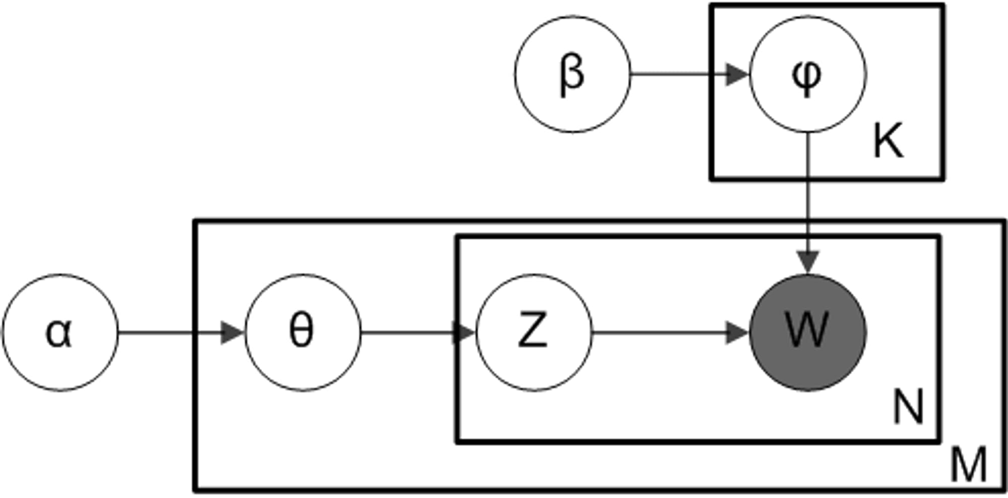
Topic models are generally represented by a plate-notation diagram as shown below source. The rectangles (also called plates in the diagram) represent loops, while the circles represent variables. The $\alpha$ and $\beta$ priors are consumed by $\Theta$ and $\Phi$ representing document-topic and topic-word distributions, respectively. W represents the sampled word, while Z is the topic assigned to it. K, M, and N are the loop stopping conditions representing the number of topics, the number of documents in the corpus, and the number of words in the topics, respectively. It can also be observed that among all variables, only W has a gray background, as it is the only known variable.

$\Theta{d, t} = \frac{\eta{d, t}^{-} + \alpha}{\sum{k}^{K} \eta{d,k}^{-} + K\alpha}$

and

$\Phi{t, w} = \frac{\eta{t, w}^{-} + \beta}{\sum{v}^{V} \eta{t,v}^{-} + V\beta}$

$P(z = t | z-, w, d, .) = \Theta{d, t} \times \Phi_{t, w}$

Where, w is the sampled word from d^{th} document, whose probability is computed for topic t in $\Theta{d, t}$. The denominator normalizes the probabilities, having K as the total number of topics. $\Phi{t, w}$ computes the probability of word w for topic t, where V is the vocabulary size. $\eta$ represents frequency e.g., $\eta_{d,t}$ means the number of times topic t appears in document d. While - is for excluding the scores of the sampled word to avoid bias in favor of the present topic.

The Vanilla implementation offers higher transparency and thus more control over the internal decisions of the method.

Contact details

M. Taimoor Khan (taimoor.khan@gesis.org)