adaptiveresonancelib
An expansive and modular collection of ART models
Science Score: 54.0%
This score indicates how likely this project is to be science-related based on various indicators:
-
✓CITATION.cff file
Found CITATION.cff file -
✓codemeta.json file
Found codemeta.json file -
✓.zenodo.json file
Found .zenodo.json file -
○DOI references
-
○Academic publication links
-
✓Committers with academic emails
1 of 2 committers (50.0%) from academic institutions -
○Institutional organization owner
-
○JOSS paper metadata
-
○Scientific vocabulary similarity
Low similarity (11.0%) to scientific vocabulary
Repository
An expansive and modular collection of ART models
Basic Info
- Host: GitHub
- Owner: NiklasMelton
- License: mit
- Language: Python
- Default Branch: develop
- Size: 2.45 MB
Statistics
- Stars: 24
- Watchers: 3
- Forks: 6
- Open Issues: 11
- Releases: 7
Metadata Files
README.md
AdaptiveResonanceLib
Welcome to AdaptiveResonanceLib, a comprehensive and modular Python library for Adaptive Resonance Theory (ART) algorithms. Based on scikit-learn, our library offers a wide range of ART models designed for both researchers and practitioners in the field of machine learning and neural networks. Whether you're working on classification, clustering, or pattern recognition, AdaptiveResonanceLib provides the tools you need to implement ART algorithms efficiently and effectively.
//: # ()
//: # ()
Adaptive Resonance Theory (ART)
Adaptive Resonance Theory (ART) is both 1. A neuroscientific theory of how the brain balances plasticity (learning new information) with stability (retaining what it already knows), and 2. A family of machine‑learning algorithms that operationalise this idea for clustering, classification, continual‑learning, and other tasks.
First proposed by Stephen Grossberg and Gail Carpenter in the mid‑1970s , ART models treat learning as an interactive search between bottom‑up evidence and top‑down expectations:
Activation. A new input pattern activates stored memories (categories) in proportion to their similarity to the input.
Candidate selection. The most active memory (call it J) is tentatively chosen to represent the input.
Vigilance check (resonance test). The match between the input and memory J is compared to a user‑chosen threshold (ρ) (the vigilance parameter).
- If the match ≥ (ρ) → Resonance. The memory and input are deemed compatible; J is updated to incorporate the new information.
- If the match < (ρ) → Mismatch‑reset. Memory J is temporarily inhibited, and the next best candidate is tested.
- If no memory passes the test → a new category is created directly from the input.
Output. In clustering mode, the index of the resonant (or newly created) memory is returned as the cluster label.
Vigilance
ρ sets an explicit upper bound on how dissimilar two inputs can be while still ending up in the same category:
| Vigilance (ρ) | Practical effect | |-----------------------------|------------------| | ( ρ = 0 ) | All inputs merge into a single, broad category | | Moderate (( 0 < ρ < 1 )) | Finer granularity as (ρ) increases | | ( ρ = 1 ) | Every distinct input forms its own category (memorisation) |
This single knob lets practitioners trade off specificity against generality without retraining from scratch.
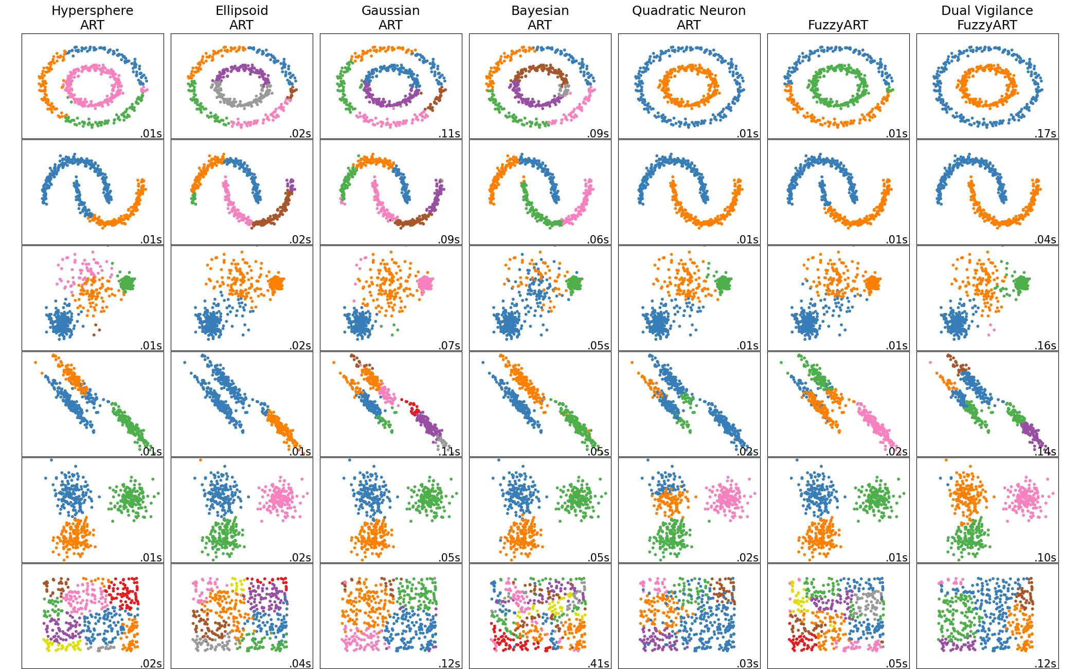
Notable Variants
| Variant | Input type | Task | Trait | |----------------------------------|-------------------------------------------|---------------------------|------------------------------------------------------------------------------------------------| | ART 1 | Binary | Unsupervised clustering | Original model | | Fuzzy ART | Real‑valued ([0,1]) | Unsupervised clustering | Uses fuzzy AND operator for analog inputs, resulting in rectagular categories | | ARTMAP | Paired inputs ((X, y)) | Supervised classification | Two ART modules linked by an associative map field | | Gaussian ART | Real‑valued | Clustering | Replace rectangular category fields with Gaussian ones for smoother decision boundaries | | FALCON | Paired inputs ((State, Action, Reward)) | Reinforcement Learning | Uses three ART modules to create a dynamic SARSA grid for solving reinforcement learning tasks |
All variants share the same resonance‑test backbone, so you can grasp one and quickly extend to the others.
Strengths and Things to Watch
- Online / incremental learning – adapts one sample at a time without replay.
- Explicit category prototypes – easy to inspect and interpret.
- Built‑in catastrophic‑forgetting control via (ρ).
- Parameter sensitivity – vigilance (and, in many variants, the learning rate (\beta)) must be tuned to your data.
- Order dependence – the sequence of inputs can affect category formation; shuffling your training data is recommended for unbiased results. <!-- END what is ART -->
Available Models
AdaptiveResonanceLib includes implementations for the following ART models:
- #### Elementary Clustering
- #### Metric Informed
- #### Topological
- #### Classification
- #### Regression
- #### Hierarchical
- #### Data Fusion
- #### Reinforcement Learning
- #### Biclustering
- #### C++ Accelerated
- Binary Fuzzy ARTMAP
Comparison of Elementary Models
[comment]: <> ()
 <!-- END comparisonofelementary_models -->
Installation
To install AdaptiveResonanceLib, simply use pip:
bash
pip install artlib
Or to install directly from the most recent source:
bash
pip install git+https://github.com/NiklasMelton/AdaptiveResonanceLib.git@develop
Ensure you have Python 3.9 or newer installed. <!-- END installation -->
Quick Start
Here are some quick examples to get you started with AdaptiveResonanceLib:
Clustering Data with the Fuzzy ART model
```python from artlib import FuzzyART import numpy as np from tensorflow.keras.datasets import mnist
Load the MNIST dataset
ndim = 28*28 (Xtrain, ), (Xtest, ) = mnist.loaddata() Xtrain = Xtrain.reshape((-1, ndim)) # flatten images Xtest = Xtest.reshape((-1, ndim))
Initialize the Fuzzy ART model
model = FuzzyART(rho=0.7, alpha = 0.0, beta=1.0)
(Optional) Tell the model the data limits for normalization
lowerbounds = np.array([0.]*ndim) upperbounds = np.array([255.]*ndim) model.setdatabounds(lowerbounds, upperbounds)
Prepare Data
trainXprep = model.preparedata(Xtrain) testXprep = model.preparedata(Xtest)
Fit the model
model.fit(trainXprep)
Predict data labels
predictions = model.predict(testXprep) ```
Fitting a Classification Model with SimpleARTMAP
```python from artlib import GaussianART, SimpleARTMAP import numpy as np from tensorflow.keras.datasets import mnist
Load the MNIST dataset
ndim = 28*28 (Xtrain, ytrain), (Xtest, ytest) = mnist.loaddata() Xtrain = Xtrain.reshape((-1, ndim)) # flatten images Xtest = Xtest.reshape((-1, ndim))
Initialize the Gaussian ART model
sigmainit = np.array([0.5]*Xtrain.shape[1]) # variance estimate for each feature modulea = GaussianART(rho=0.0, sigmainit=sigma_init)
(Optional) Tell the model the data limits for normalization
lowerbounds = np.array([0.]*ndim) upperbounds = np.array([255.]*ndim) modulea.setdatabounds(lowerbounds, upper_bounds)
Initialize the SimpleARTMAP model
model = SimpleARTMAP(modulea=modulea)
Prepare Data
trainXprep = model.preparedata(Xtrain) testXprep = model.preparedata(Xtest)
Fit the model
model.fit(trainXprep, y_train)
Predict data labels
predictions = model.predict(testXprep) ```
Fitting a Regression Model with FusionART
```python from artlib import FuzzyART, HypersphereART, FusionART import numpy as np
Your dataset
Xtrain = np.array([...]) # shape (nsamples, nfeaturesX) ytrain = np.array([...]) # shape (nsamples, nfeaturesy) test_X = np.array([...])
Initialize the Fuzzy ART model
module_x = FuzzyART(rho=0.0, alpha = 0.0, beta=1.0)
Initialize the Hypersphere ART model
rhat = 0.5*np.sqrt(Xtrain.shape[1]) # no restriction on hyperpshere size moduley = HypersphereART(rho=0.0, alpha = 0.0, beta=1.0, rhat=r_hat)
Initialize the FusionARTMAP model
gammavalues = [0.5, 0.5] # eqaul weight to both channels channeldims = [ 2X_train.shape[1], # fuzzy ART complement codes data so channel dim is 2nfeatures ytrain.shape[1] ] model = FusionART( modules=[modulex, moduley], gammavalues=gammavalues, channeldims=channeldims )
Prepare Data
trainXy = model.joinchanneldata(channeldata=[Xtrain, ytrain]) trainXyprep = model.preparedata(trainXy) testXy = model.joinchanneldata(channeldata=[Xtrain], skipchannels=[1]) testXyprep = model.preparedata(testXy)
Fit the model
model.fit(trainXyprep)
Predict y-channel values and clip X values outside previously observed ranges
predy = model.predictregression(testXyprep, target_channels=[1], clip=True) ```
Data Normalization
AdaptiveResonanceLib models require feature data to be normalized between 0.0 and 1.0 inclusively. This requires identifying the boundaries of the data space.
If the first batch of your training data is representative of the entire data space, you dont need to do anything and artlib will identify the data bounds automatically. However, this will often not be sufficient and the following work-arounds will be needed:
Users can manually set the bounds using the following code snippet or similar: ```python
Set the boundaries of your data for normalization
lowerbounds = np.array([0.]*nfeatures) upperbounds = np.array([1.]*nfeatures) model.setdatabounds(lowerbounds, upperbounds) ```
Or users can present all batches of data to the model for automatic boundary identification: ```python
Find the boundaries of your data for normalization
alldata = [trainX, testX] _, _ = model.finddatabounds(alldata) ```
If only the boundaries of your testing data are unknown, you can call
model.predict() with clip=True to clip testing data to the bounds seen during
training. Only use this if you understand what you are doing.
//: # ()
//: # ()
//: # ()
//: # ()
//: # ()
C++ Optimizations
Most ARTlib classes rely on NumPy / SciPy for linear-algebra routines, but several go further:
| Level | Accelerated components | Implementations | |-------|------------------------|-----------------| | Python (Numba JIT) | Activation & vigilance kernels | ART1, Fuzzy ART, Binary Fuzzy ART | | Native C++ (Pybind11) | Entire fit / predict pipelines | Fuzzy ARTMAP, Hypersphere ARTMAP, Gaussian ARTMAP, Binary Fuzzy ARTMAP |
How the C++ variants work
- End-to-end native execution – Training and inference run entirely in C++, eliminating Python-level overhead.
- State hand-off – After fitting, the C++ routine exports cluster weights and metadata back to the corresponding pure-Python class. You can therefore:
• inspect attributes (
weights_,categories_, …) • serialize withpickle• plug them into any downstream ARTlib or scikit-learn pipeline exactly as you would with the Python-only models. - Trade-off – The C++ versions sacrifice some modularity (you cannot swap out internal ART components) in exchange for significantly shorter run-times.
C++ Acceleration Quick reference
| Class | Acceleration method | Primary purpose | |-----------------------|---------------------------|-----------------| | ART1 | Numba JIT kernels | Clustering | | Fuzzy ART | Numba JIT kernels | Clustering | | Binary Fuzzy ART | Numba JIT kernels | Clustering | | | | | | Fuzzy ARTMAP | Full C++ implementation | Classification | | Hypersphere ARTMAP | Full C++ implementation | Classification | | Gaussian ARTMAP | Full C++ implementation | Classification | | Binary Fuzzy ARTMAP | Full C++ implementation | Classification |
Example Usage
```python from artlib import FuzzyARTMAP import numpy as np from tensorflow.keras.datasets import mnist
Load the MNIST dataset
ndim = 28*28 (Xtrain, ytrain), (Xtest, ytest) = mnist.loaddata() Xtrain = Xtrain.reshape((-1, ndim)) # flatten images Xtest = Xtest.reshape((-1, ndim))
Initialize the Fuzzy ART model
model = FuzzyARTMAP(rho=0.7, alpha = 0.0, beta=1.0)
(Optional) Tell the model the data limits for normalization
lowerbounds = np.array([0.]*ndim) upperbounds = np.array([255.]*ndim) model.setdatabounds(lowerbounds, upperbounds)
Prepare Data
trainXprep = model.preparedata(Xtrain) testXprep = model.preparedata(Xtest)
Fit the model
model.fit(trainXprep, y_train)
Predict data labels
predictions = model.predict(testXprep) ```
Timing Comparison
The below figures demonstrate the acceleration seen by the C++ ARTMAP variants in comparison to their baseline Python versions for a 1000 sample subset of the MNIST dataset.
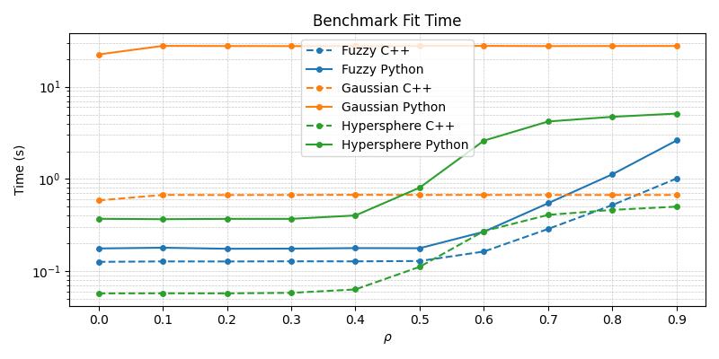
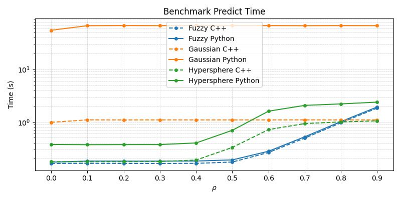
From the above plots, it becomes apparent that the C++ variants are superior in their runtime performance and should be the default choice of practitioners wishing to work with these specific compound models.
While the current selection remains limited, future releases will expand the native C++ implementation as user demand for them increases.
Documentation
For more detailed documentation, including the full list of parameters for each model, visit our Read the Docs page. <!-- END documentation -->
Examples
For examples of how to use each model in AdaptiveResonanceLib, check out the /examples directory in our repository.
<!-- END examples -->
Contributing
We welcome contributions to AdaptiveResonanceLib! If you have suggestions for improvements, or if you'd like to add more ART models, please see our CONTRIBUTING.md file for guidelines on how to contribute.
You can also join our Discord server and participate directly in the discussion. <!-- END contributing -->
License
AdaptiveResonanceLib is open source and available under the MIT license. See the LICENSE file for more info.
<!-- END license -->
Contact
For questions and support, please open an issue in the GitHub issue tracker or message us on our Discord server. We'll do our best to assist you.
Happy Modeling with AdaptiveResonanceLib! <!-- END contact -->
Citing this Repository
If you use this project in your research, please cite it as:
Melton, N. (2024). AdaptiveResonanceLib (Version 0.1.6) <!-- END citation -->
Owner
- Login: NiklasMelton
- Kind: user
- Repositories: 1
- Profile: https://github.com/NiklasMelton
JOSS Publication
Adaptive Resonance Lib: A Python package for Adaptive Resonance Theory (ART) models
Authors

Missouri University of Science and Technology, Rolla, Missouri, United States of America
Missouri University of Science and Technology, Rolla, Missouri, United States of America
Missouri University of Science and Technology, Rolla, Missouri, United States of America
Editor
Marcel Stimberg
Tags
python clustering classification regression reinforcement learning machine learningCitation (CITATION.cff)
cff-version: 1.2.0
message: "If you use this software, please cite it as below."
title: "AdaptiveResonanceLib"
version: "0.1.6"
doi: "10.5281/zenodo.9999999"
authors:
  - family-names: "Melton"
    given-names: "Niklas"
    orcid: "https://orcid.org/0000-0001-9625-7086"
date-released: 2024-10-03
url: "https://github.com/NiklasMelton/AdaptiveResonanceLib"
repository-code: "https://github.com/NiklasMelton/AdaptiveResonanceLib"
license: "MIT"
keywords:
  - "adaptive resonance theory"
  - "ART"
  - "machine learning"
  - "clustering"
  - "neural networks"
GitHub Events
Total
- Create event: 60
- Issues event: 6
- Release event: 7
- Watch event: 16
- Delete event: 57
- Issue comment event: 9
- Push event: 314
- Pull request event: 124
- Fork event: 2
Last Year
- Create event: 60
- Issues event: 6
- Release event: 7
- Watch event: 16
- Delete event: 57
- Issue comment event: 9
- Push event: 314
- Pull request event: 124
- Fork event: 2
Committers
Last synced: over 1 year ago
Top Committers
| Name | Commits | |
|---|---|---|
| niklas melton | n****n@g****m | 255 |
| Dustin Tanksley | d****9@u****u | 1 |
Committer Domains (Top 20 + Academic)
Issues and Pull Requests
Last synced: 10 months ago
All Time
- Total issues: 27
- Total pull requests: 238
- Average time to close issues: 3 days
- Average time to close pull requests: about 8 hours
- Total issue authors: 3
- Total pull request authors: 2
- Average comments per issue: 0.67
- Average comments per pull request: 0.01
- Merged pull requests: 217
- Bot issues: 0
- Bot pull requests: 0
Past Year
- Issues: 5
- Pull requests: 136
- Average time to close issues: 7 days
- Average time to close pull requests: about 10 hours
- Issue authors: 3
- Pull request authors: 2
- Average comments per issue: 1.0
- Average comments per pull request: 0.01
- Merged pull requests: 116
- Bot issues: 0
- Bot pull requests: 0
Top Authors
Issue Authors
- NiklasMelton (25)
- TahiriNadia (1)
- cleong110 (1)
Pull Request Authors
- NiklasMelton (234)
- DustinTanksley (4)