SCGraph

<!-- -->

A Supply chain graph package for Python

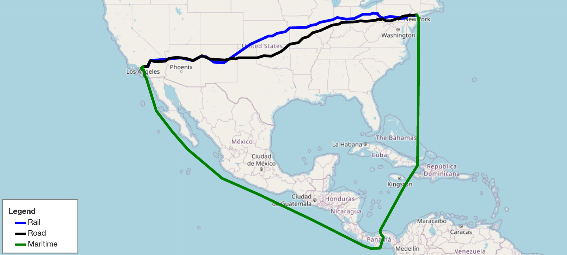
Quick Start:

Get the shortest maritime path length between Shanghai, China and Savannah, Georgia, USA ```py

Use a maritime network geograph

from scgraph.geographs.marnet import marnetgeograph output = marnetgeograph.getshortestpath( originnode={"latitude": 31.23,"longitude": 121.47}, destinationnode={"latitude": 32.08,"longitude": -81.09}, output_units='km', ) print('Length: ',output['length']) #=> Length: 19596.4653 ```

Documentation

• Docs: https://connor-makowski.github.io/scgraph/scgraph.html
• Git Repo: https://github.com/connor-makowski/scgraph
• Paper: https://ssrn.com/abstract=5388845

How to Cite SCGraph in your Research

If you use SCGraph for your research, please consider citing the following paper:

Makowski, C., Saragih, A., Guter, W., Russell, T., Heinold, A., & Lekkakos, S. (2025). SCGraph: A dependency-free Python package for road, rail, and maritime shortest path routing generation and distance estimation. MIT Center for Transportation & Logistics Research Paper Series, (2025-028). https://ssrn.com/abstract=5388845

Or by using the BibTeX entry:

@article{makowski2025scgraph, title={SCGraph: A Dependency-Free Python Package for Road, Rail, and Maritime Shortest Path Routing Generation and Distance Estimation}, author={Makowski, Connor and Saragih, Austin and Guter, Willem and Russell, Tim and Heinold, Arne and Lekkakos, Spyridon}, journal={MIT Center for Transportation \& Logistics Research Paper Series}, number={2025-028}, year={2025}, url={https://ssrn.com/abstract=5388845} }

Getting Started

Installation

pip install scgraph

Basic Geograph Usage

Get the shortest path between two points on earth using a latitude / longitude pair.

In this case, calculate the shortest maritime path between Shanghai, China and Savannah, Georgia, USA.

```py

Use a maritime network geograph

from scgraph.geographs.marnet import marnet_geograph

Note: The origin and destination nodes can be any latitude / longitude pair

output = marnetgeograph.getshortestpath( originnode={"latitude": 31.23,"longitude": 121.47}, destinationnode={"latitude": 32.08,"longitude": -81.09}, outputunits='km', # Optional: Cache the origin node's spanning tree for faster calculations on future calls from the same origin node when cache=True # Note: This will make the first call slower, but future calls using this origin node will be substantially faster. cache=True, ) print('Length: ',output['length']) #=> Length: 19596.4653 ```

Adding in a few additional parameters to the get_shortest_path function can change the output format as well as performance of the calculation. ```py

Use a maritime network geograph

from scgraph.geographs.marnet import marnet_geograph

Get the shortest maritime path between Shanghai, China and Savannah, Georgia, USA

output = marnetgeograph.getshortestpath( originnode={"latitude": 31.23,"longitude": 121.47}, destinationnode={"latitude": 32.08,"longitude": -81.09}, outputunits='km', nodeadditionlatlonbound=180, # Optional: The maximum distance in degrees to consider nodes when attempting to add the origin and destination nodes to the graph nodeadditiontype='quadrant', # Optional: Instead of connecting the origin node to the graph by the closest node, connect it to the closest node in each direction (NE, NW, SE, SW) if found within the nodeadditionlatlonbound destinationnodeadditiontype='all', # Optional: Instead of connecting the destination node to the graph by the closest node, connect it to all nodes found within the nodeadditionlatlonbound # When destinationnodeadditiontype='all' is set with a nodeadditionlatlonbound=180, this will guarantee a solution can be found since the destination node will also connect to the origin node ) print('Length: ',output['length']) #=> Length: 19596.4653 ```

In the above example, the output variable is a dictionary with two keys: length and coordinate_path.

• length: The distance between the passed origin and destination when traversing the graph along the shortest path
  • Notes:
    • This will be in the units specified by the output_units parameter.
    • output_units options:
      • km (kilometers - default)
      • m (meters)
      • mi (miles)
      • ft (feet)
• coordinate_path: A list of lists [latitude,longitude] that make up the shortest path

You can also select a different algorithm function for the shortestpath: ```py from scgraph.geographs.marnet import marnetgeograph from scgraph import Graph output = marnetgeograph.getshortestpath( originnode={"latitude": 31.23,"longitude": 121.47}, destinationnode={"latitude": 32.08,"longitude": -81.09}, # Optional: Specify an algorithmfn to call when solving the shortestpath algorithmfn=Graph.bmssp, ) ```

Don't neglect the very efficient distance matrix function to quickly get the distances between multiple points on the graph. Each origin graph entry point and spanning tree is cached so you can generate massive distance matricies incredibly quickly (approaching 50 nano seconds per distance for large enough distance matricies). ```py from scgraph.geographs.usfreeway import usfreeway_geograph

cities = [ {"latitude": 34.0522, "longitude": -118.2437}, # Los Angeles {"latitude": 40.7128, "longitude": -74.0060}, # New York City {"latitude": 41.8781, "longitude": -87.6298}, # Chicago {"latitude": 29.7604, "longitude": -95.3698}, # Houston ]

distancematrix = usfreewaygeograph.distancematrix(cities, output_units='km')

[

[0.0, 4510.965665644833, 3270.3864033755776, 2502.886438995942],

[4510.9656656448415, 0.0, 1288.473118634311, 2637.5821542546687],

[3270.3864033755744, 1288.4731186343113, 0.0, 1913.1928919854067],

[2502.886438995935, 2637.5821542546687, 1913.1928919854076, 0.0],

]

```

For more examples including viewing the output on a map, see the example notebook.

Examples with Google Colab

• Getting Started
• Creating A Multi Path Geojson
• Modifying A Geograph

GridGraph usage

Example: - Create a grid of 20x20 cells. - This creates a grid based graph with connections to all 8 neighbors for each grid item. - Each grid item has 4 cardinal connections at length 1 and 4 diagonal connections at length sqrt(2) - Create a wall from (10,5) to (10,19). - This would foce any path to go to the bottom of the graph to get around the wall. - Get the shortest path between (2,10) and (18,10) - Note: The length of this path should be 16 without the wall and 20.9704 with the wall.

```py from scgraph import GridGraph

xsize = 20 ysize = 20 blocks = [(10, i) for i in range(5, y_size)]

Create the GridGraph object

gridGraph = GridGraph( xsize=xsize, ysize=ysize, blocks=blocks, addexteriorwalls=True, )

Solve the shortest path between two points

output = gridGraph.getshortestpath( originnode={"x": 2, "y": 10}, destinationnode={"x": 18, "y": 10}, # Optional: Specify the output coodinate format (default is 'listofdicts) outputcoordinatepath="listoflists", # Optional: Cache the origin point spanning_tree for faster calculations on future calls cache=True, )

print(output)

=> {'length': 20.9704, 'coordinate_path': [[2, 10], [3, 9], [4, 8], [5, 8], [6, 7], [7, 6], [8, 5], [9, 4], [10, 4], [11, 4], [12, 5], [13, 6], [14, 7], [15, 7], [16, 8], [17, 9], [18, 10]]}

```

About

Key Features

• Graph:
  • A low level graph object that has methods for validating graphs, calculating shortest paths, and more.
  • See: Graph Documentation
  • Contains the following methods:
    • validate_graph: Validates symmetry and connectedness of a graph.
    • dijkstra: Calculates the shortest path between two nodes using Dijkstra's algorithm.
    • dijkstra_makowski: Calculates the shortest path between two nodes using a modified version of Dijkstra's algorithm designed for real world performance
    • dijkstra_negative: Calculates the shortest path between two nodes using a modified version of Dijkstra's algorithm that supports negative edge weights and detects negative cycles.
    • a_star: Modified version of dijkstra_makowski that incorporates a heuristic function to guide the search.
    • bellman_ford: Calculates the shortest path between two nodes using the Bellman-Ford algorithm.
    • bmssp: Calculates the shortest path between two nodes using a modified version of the BMSSP Algorithm. See the BmsspSolver.
• GeoGraphs:
  • A geographic graph data structure that allows for the calculation of shortest paths between two points on earth
  • Uses latitude / longitude pairs to represent points on earth
  • Supports maritime, rail, road and other geographic networks
  • Uses a sparse network data structure to represent the graph
  • How to use it - Calculate the shortest path between two points on earth
    • Inputs:
      • A latitude / longitude pair for the origin
      • A latitude / longitude pair for the destination
    • Calculation:
      • See the Graph documentation above for available algorithms.
    • Returns:
      • path:
        • A list of lists [latitude, longitude] that make up the shortest path
      • length:
        • The distance (in the units requested) between the two points
  • Precompiled Geographs offer Antimeridian support
  • Arbitrary start and end points are supported
    • Start and end points do not need to be in the graph
  • Cached shortest path calculations can be used for very fast repetative calculations from the same origin node in a GeoGraph.
    • This is done by caching the origin node's spanning tree
    • The first call will be slower, but future calls using this origin node will be substantially faster.
• GridGraphs:
  • A grid based graph data structure that allows for the calculation of shortest paths between two points on a grid
  • See: GridGraph Documentation
  • Supports arbitrary grid sizes and blockages
  • Uses a sparse network data structure to represent the graph
  • How to use it - Calculate the shortest path between two points on a grid
    • Inputs:
      • A (x,y) coordinate on the grid for the origin
      • A (x,y) coordinate on the grid for the destination
    • Calculation:
      • Algorithms:
        • Dijkstra's algorithm
        • Modified Dijkstra algorithm
        • A* algorithm (Extension of the Modified Dijkstra)
    • Returns:
      • length:
        • The distance between the two points on the grid
      • coordinate_path:
        • A list of dicts {"x": x, "y": y} representing the path taken through the grid
  • Arbitrary start and end points are supported
    • Start and end points do not need to be in the graph
  • Arbitrary connection matricies are supported
    • Cardinal connections (up, down, left, right) and diagonal connections (up-left, up-right, down-left, down-right) are used by default
    • Custom connection matricies can be used to change the connections between grid items
  • Cached shortest path calculations can be used for very fast repetative calculations to or from the same point in a GridGraph.
• Other Useful Features:
  • CacheGraphs:
    • A graph extension that caches spanning trees for fast shortest path calculations on repeat calls from the same origin node
    • See: CacheGraphs Documentation
  • SpanningTrees:
    • See: Spanning Trees Documentation

Included GeoGraphs

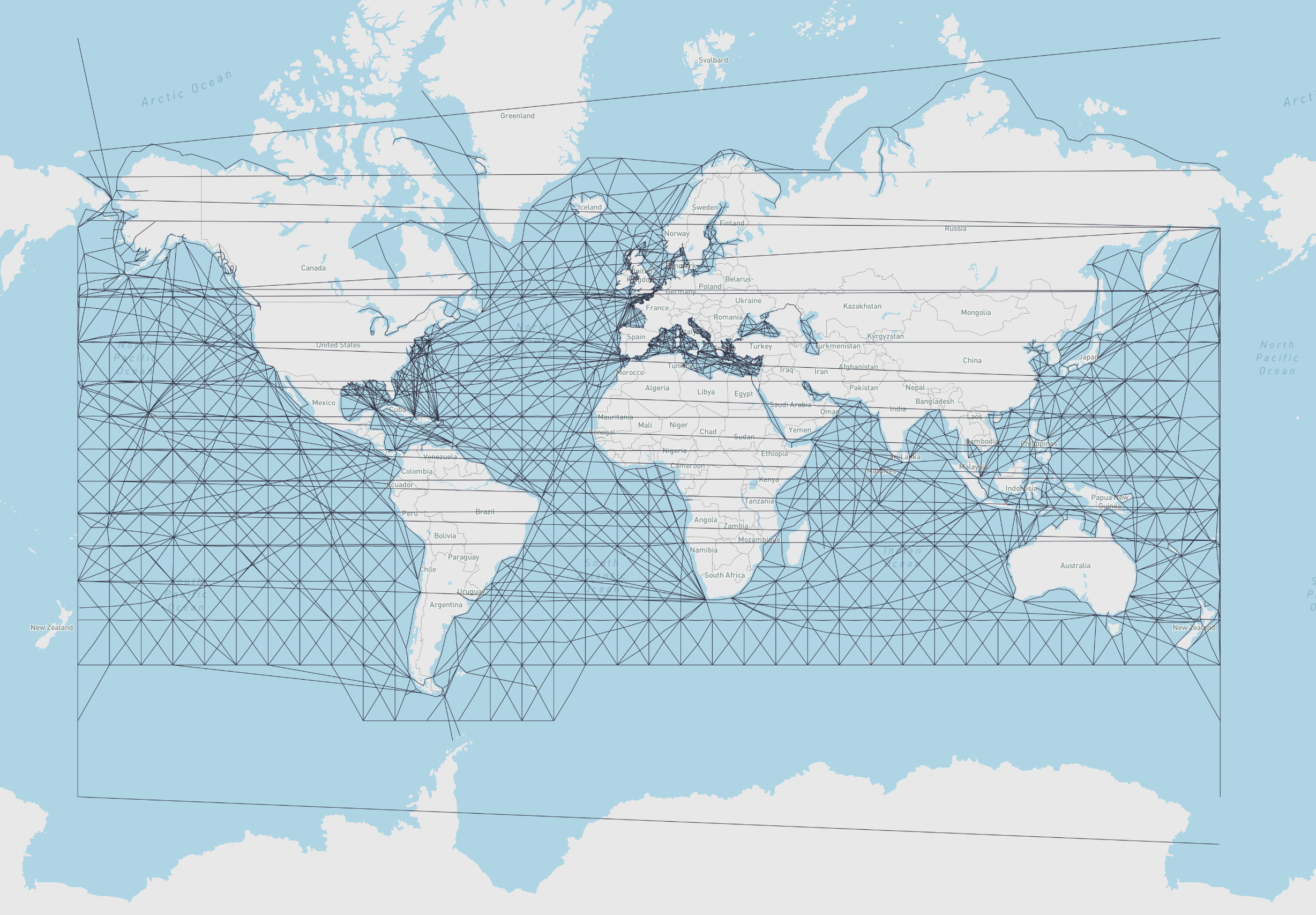
• marnet_geograph:
  • What: A maritime network data set from searoute
  • Use: from scgraph.geographs.marnet import marnet_geograph
  • Attribution: searoute
  • Length Measurement: Kilometers
  • Marnet Picture
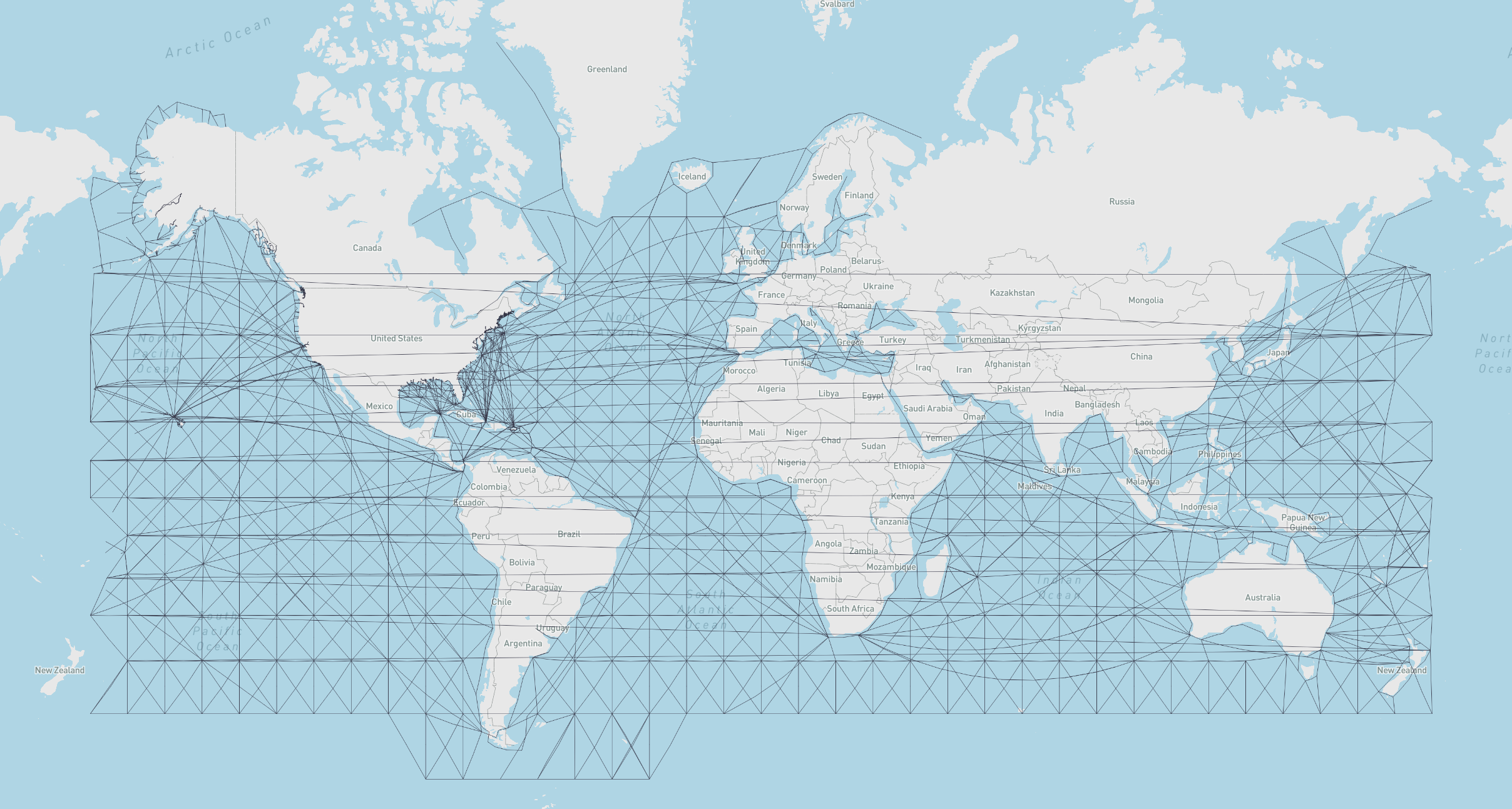
• oakridgemaritime_geograph:
  • What: A maritime data set from the Oak Ridge National Laboratory campus
  • Use: from scgraph.geographs.oak_ridge_maritime import oak_ridge_maritime_geograph
  • Attribution: Oak Ridge National Laboratory with data from Geocommons
  • Length Measurement: Kilometers
  • Oak Ridge Maritime Picture
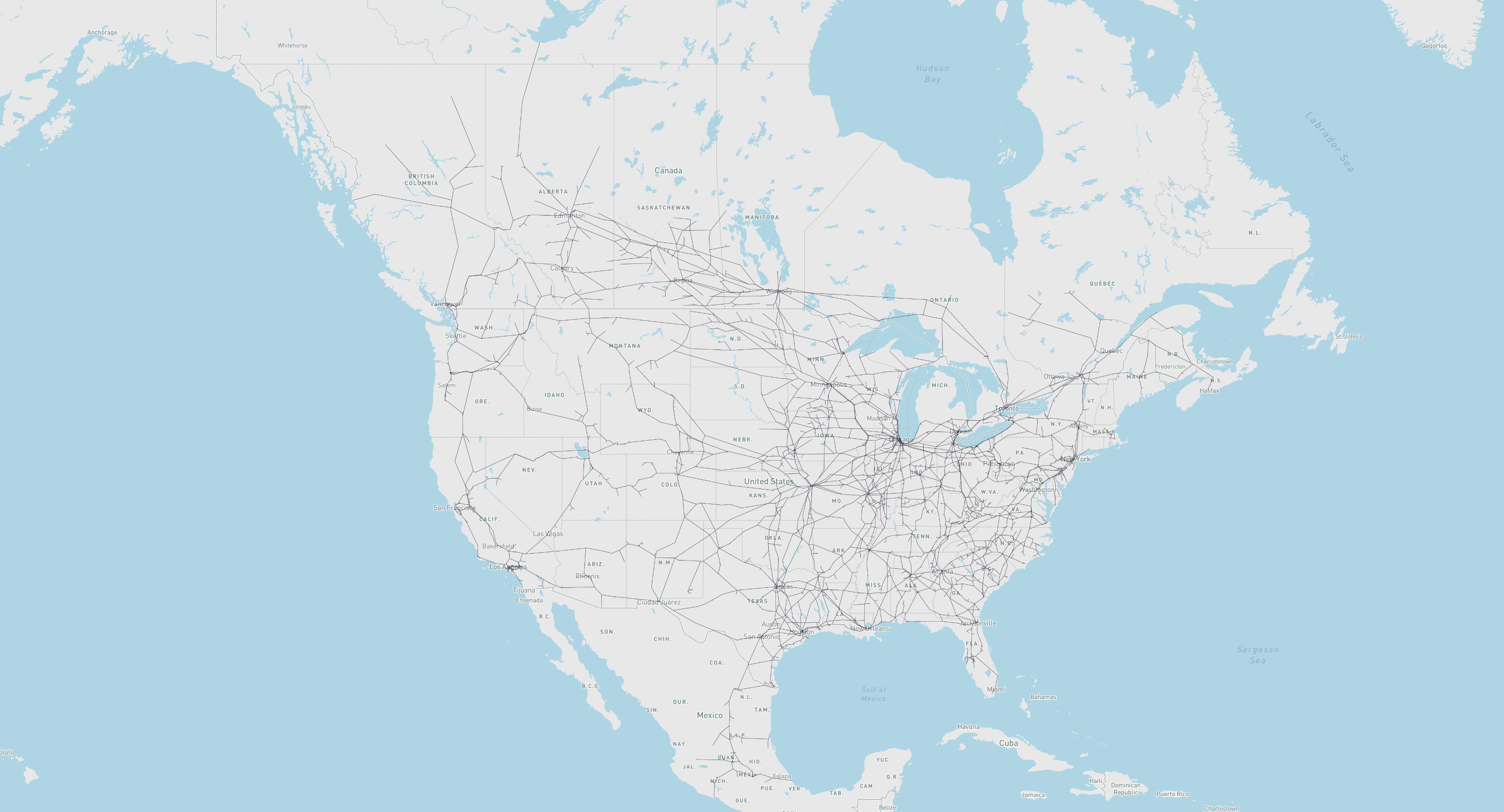
• northamericarail_geograph:
  • What: Class 1 Rail network for North America
  • Use: from scgraph.geographs.north_america_rail import north_america_rail_geograph
  • Attribution: U.S. Department of Transportation: ArcGIS Online
  • Length Measurement: Kilometers
  • North America Rail Picture
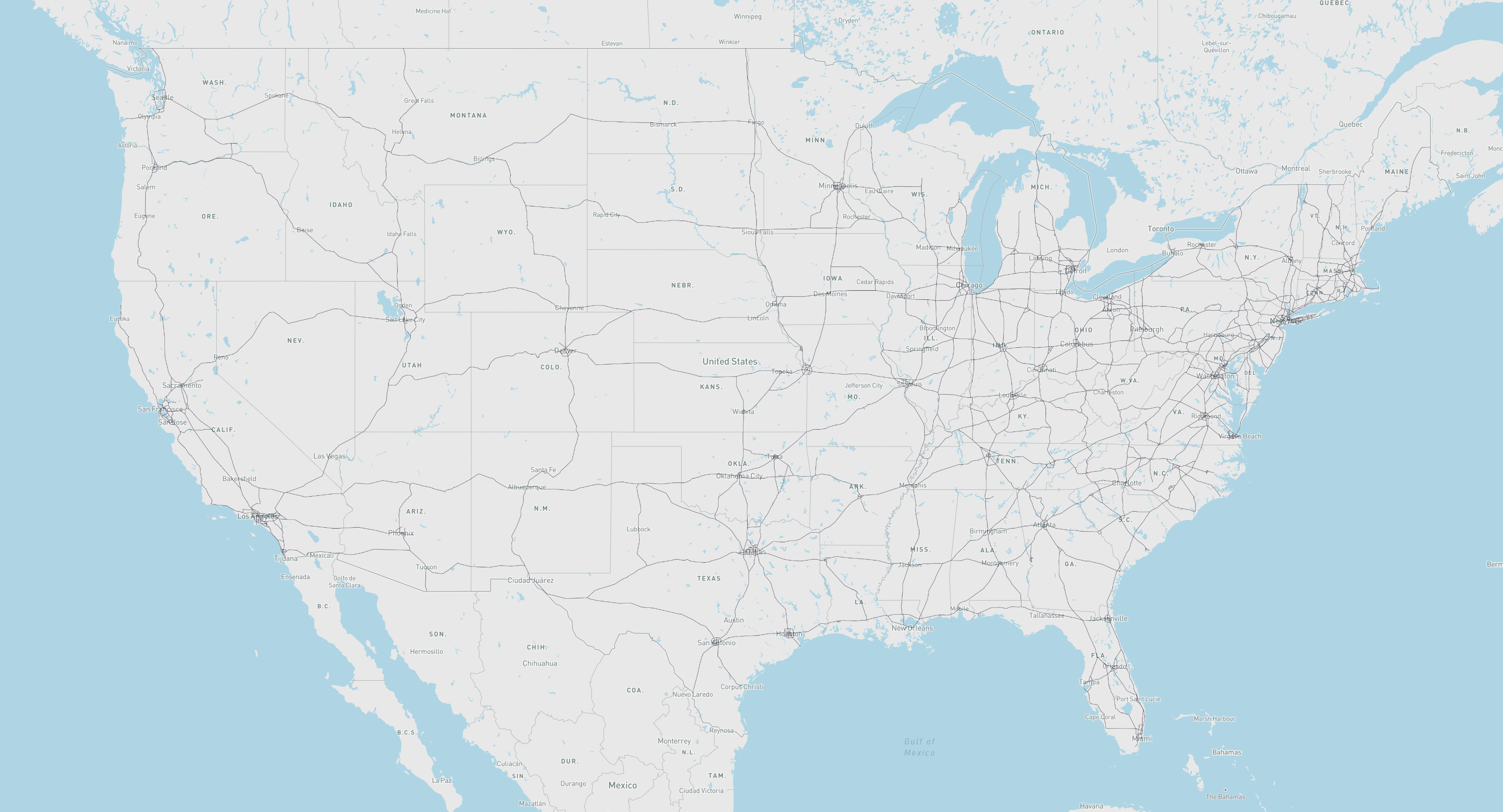
• usfreewaygeograph:
  • What: Freeway network for the United States
  • Use: from scgraph.geographs.us_freeway import us_freeway_geograph
  • Attribution: U.S. Department of Transportation: ArcGIS Online
  • Length Measurement: Kilometers
  • US Freeway Picture
• scgraph_data geographs:
  • What: Additional geographs are available in the scgraph_data package
    • Note: These include larger geographs like the world highways geograph and world railways geograph.
  • Installation: pip install scgraph_data
  • Use: from scgraph_data.world_highways import world_highways_geograph
  • See: scgraph_data for more information and all available geographs.
• Custom Geographs:
  • What: Users can create their own geographs from various data sources
  • See: Building your own Geographs from Open Source Data

Advanced Usage

Using scgraph_data geographs

Using scgraph_data geographs: - Note: Make sure to install the scgraph_data package before using these geographs ```py from scgraphdata.worldrailways import worldrailwaysgeograph from scgraph import Graph

Get the shortest path between Kalamazoo Michigan and Detroit Michigan by Train

output = worldrailwaysgeograph.getshortestpath( originnode={"latitude": 42.29,"longitude": -85.58}, destinationnode={"latitude": 42.33,"longitude": -83.05}, # Optional: Use the A* algorithm algorithmfn=Graph.astar, # Optional: Pass the haversine function as the heuristic function to the A* algorithm algorithmkwargs={"heuristicfn": worldrailwaysgeograph.haversine}, ) ```

Building your own Geographs from Open Source Data

You can build your own geographs using various tools and data sources. For example, you can use OpenStreetMap data to create a high fidelity geograph for a specific area.

Follow this step by step guide on how to create a geograph from OpenStreetMap data. For this example, we will use some various tools to create a geograph for highways (including seconday highways) in Michigan, USA.

Download an OSM PBF file using the AWS CLI: - Geofabrik is a good source for smaller OSM PBF files. See: https://download.geofabrik.de/ - To keep things generalizable, you can also download the entire planet OSM PBF file using AWS. But you should consider downloading a smaller region if you are only interested in a specific area. - Note: For this, you will need to install the AWS CLI. - Note: The planet OSM PBF file is very large (About 100GB) aws s3 cp s3://osm-pds/planet-latest.osm.pbf . - Use Osmium to filter and extract the highways from the OSM PBF file. - Install osmium on macOS: brew install osmium-tool - Install osmium on Ubuntu: sudo apt-get install osmium-tool - Download a Poly file for the area you are interested in. This is a polygon file that defines the area you want to extract from the OSM PBF file. - For Michigan, you can download the poly file from Geofabrik: curl https://download.geofabrik.de/north-america/us/michigan.poly > michigan.poly - Google around to find an appropriate poly file for your area of interest. - Filter and extract as GeoJSON (EG: Michigan) substituting the poly and pbf file names as needed: osmium extract -p michigan.poly --overwrite -o michigan.osm.pbf planet-latest.osm.pbf - Filter the OSM PBF file to only areas of interest and export to GeoJSON: - See: https://wiki.openstreetmap.org/wiki/ - EG For Highways, see: https://wiki.openstreetmap.org/wiki/Key:highway osmium tags-filter michigan.osm.pbf w/highway=motorway,trunk,primary,motorway_link,trunk_link,primary_link,secondary,secondary_link,tertiary,tertiary_link -t --overwrite -o michigan_roads.osm.pbf osmium export michigan_roads.osm.pbf -f geojson --overwrite -o michigan_roads.geojson

• Simplify the geojson
  • This uses some tools in the SCGraph library as well as Mapshaper to simplify the geojson files.
  • Mapshaper is a CLI and web tool for simplifying and editing geojson files.
  • To install Mapshaper for CLI use, use NPM: npm install -g mapshaper
  • Mapshaper is particularly helpful since it repairs intersections in the lines which is crutial for geographs to work properly.
  • Mapshaper, however, does not handle larger files very well, so it is recommended to simplify the geojson file first using the scgraph.helpers.geojson.simplify_geojson function first to reduce the size of the file.
  • Make sure to tailor the parameters to your needs. python -c "from scgraph.helpers.geojson import simplify_geojson; simplify_geojson('michigan_roads.geojson', 'michigan_roads_simple.geojson', precision=4, pct_to_keep=100, min_points=3, silent=False)" mapshaper michigan_roads_simple.geojson -simplify 10% -filter-fields -o force michigan_roads_simple.geojson mapshaper michigan_roads_simple.geojson -snap -clean -o force michigan_roads_simple.geojson
• Load the newly created geojson file as a geograph:
  • Note: The GeoGraph.load_from_geojson function is used to load the geojson file as a geograph.
  • This will create a geograph that can be used to calculate shortest paths between points on the graph. from scgraph import GeoGraph michigan_roads_geograph = GeoGraph.load_from_geojson('michigan_roads_simple.geojson')

Custom Graphs and Geographs

Modify an existing geograph: See the notebook here

You can specify your own custom graphs for direct access to the solving algorithms. This requires the use of the low level Graph class

```py from scgraph import Graph

Define an arbitrary graph

See the graph definitions here:

https://connor-makowski.github.io/scgraph/scgraph/graph.html#Graph.validate_graph

graph = [ {1: 5, 2: 1}, {0: 5, 2: 2, 3: 1}, {0: 1, 1: 2, 3: 4, 4: 8}, {1: 1, 2: 4, 4: 3, 5: 6}, {2: 8, 3: 3}, {3: 6} ]

Optional: Validate your graph

Graph.validate_graph(graph=graph)

Get the shortest path between idx 0 and idx 5

output = Graph.dijkstramakowski(graph=graph, originid=0, destination_id=5)

=> {'path': [0, 2, 1, 3, 5], 'length': 10}

```

You can also use a slightly higher level GeoGraph class to work with latitude / longitude pairs

```py from scgraph import GeoGraph

Define nodes

See the nodes definitions here:

https://connor-makowski.github.io/scgraph/scgraph/geograph.html#GeoGraph.init

nodes = [ # London [51.5074, -0.1278], # Paris [48.8566, 2.3522], # Berlin [52.5200, 13.4050], # Rome [41.9028, 12.4964], # Madrid [40.4168, -3.7038], # Lisbon [38.7223, -9.1393] ]

Define a graph

See the graph definitions here:

https://connor-makowski.github.io/scgraph/scgraph/graph.html#Graph.validate_graph

graph = [ # From London { # To Paris 1: 311, }, # From Paris { # To London 0: 311, # To Berlin 2: 878, # To Rome 3: 1439, # To Madrid 4: 1053 }, # From Berlin { # To Paris 1: 878, # To Rome 3: 1181, }, # From Rome { # To Paris 1: 1439, # To Berlin 2: 1181, }, # From Madrid { # To Paris 1: 1053, # To Lisbon 5: 623 }, # From Lisbon { # To Madrid 4: 623 } ]

Create a GeoGraph object

my_geograph = GeoGraph(nodes=nodes, graph=graph)

Optional: Validate your graph

mygeograph.validategraph()

Optional: Validate your nodes

mygeograph.validatenodes()

Get the shortest path between two points

In this case, Birmingham England and Zaragoza Spain

Since Birmingham and Zaragoza are not in the graph,

the algorithm will add them into the graph.

See: https://connor-makowski.github.io/scgraph/scgraph/geograph.html#GeoGraph.getshortestpath

Expected output would be to go from

Birmingham -> London -> Paris -> Madrid -> Zaragoza

output = mygeograph.getshortestpath( # Birmingham England originnode = {'latitude': 52.4862, 'longitude': -1.8904}, # Zaragoza Spain destination_node = {'latitude': 41.6488, 'longitude': -0.8891} ) print(output)

{

'length': 1799.4323,

'coordinate_path': [

[52.4862, -1.8904],

[51.5074, -0.1278],

[48.8566, 2.3522],

[40.4168, -3.7038],

[41.6488, -0.8891]

]

}

```

Development

Running Tests, Prettifying Code, and Updating Docs

Make sure Docker is installed and running on a Unix system (Linux, MacOS, WSL2).

• Create a docker container and drop into a shell
  • ./run.sh
• Run all tests (see ./utils/test.sh)
  • ./run.sh test
• Prettify the code (see ./utils/prettify.sh)
  • ./run.sh prettify

• Update the docs (see ./utils/docs.sh)

  • ./run.sh docs

• Note: You can and should modify the Dockerfile to test different python versions.

Attributions and Thanks

Originally inspired by searoute including the use of one of their datasets that has been modified to work properly with this package.