Spey: smooth inference for reinterpretation studies

Outline

• Installation
• What is Spey?
• Quick Start
• Developer's Guide: How to contribute to Spey

Installation

Spey can be found in PyPi library and can be downloaded using

bash pip install spey

If you like to use a specific branch, you can either use make install or pip install -e . after cloning the repository or use the following command:

bash python -m pip install --upgrade "git+https://github.com/SpeysideHEP/spey"

Note that main branch may not be the stable version.

What is Spey?

Spey is a plug-in-based statistics tool that aims to collect all likelihood prescriptions under one roof. This provides users with the workspace to freely combine different statistical models and study them through a single interface. In order to achieve a module that can be used both with statistical model prescriptions, which has been proposed in the past and will be used in the future, Spey uses a so-called plug-in system where developers can propose their statistical model prescriptions and allow Spey to use them.

What a plugin provides

A quick intro on the terminology of spey plugins in this section:

• A plugin is an external Python package that provides additional statistical model prescriptions to spey.
• Each plugin may provide one (or more) statistical model prescriptions that are accessible directly through Spey.
• Depending on the scope of the plugin, you may wish to provide additional (custom) operations and differentiability through various autodif packages such as autograd or jax. As long as they are implemented through a set of predefined function names spey can automatically detect and use them within the interface.

Finally, the name "Spey" originally comes from the Spey River, a river in the mid-Highlands of Scotland. The area "Speyside" is famous for its smooth whiskey.

Currently available plug-ins

| Accessor | Description | | --------------------------------------- | ---------------------------------------------------------------------------- | | "default.uncorrelated_background" | Constructs uncorrelated multi-bin statistical model. | | "default.correlated_background" | Constructs correlated multi-bin statistical model with Gaussian nuisances. | | "default.third_moment_expansion" | Implements the skewness of the likelihood by using third moments. | | "default.effective_sigma" | Implements the skewness of the likelihood by using asymmetric uncertainties. | | "default.poisson" | Implements simple Poisson-based likelihood without uncertainties. | | "default.normal" | Implements Normal distribution. | | "default.multivariate_normal" | Implements Multivariate normal distribution. | | "pyhf.uncorrelated_background" | Uses uncorrelated background functionality of pyhf (see spey-phyf plugin). | | "pyhf" | Uses generic likelihood structure of pyhf (see spey-phyf plugin) |

For details on all the backends, see the Plug-ins section of the documentation.

Quick Start

First one needs to choose which backend to work with. By default, spey is shipped with various types of likelihood prescriptions which can be checked via AvailableBackends function

```python import spey print(spey.AvailableBackends())

['default.correlated_background',

'default.effective_sigma',

'default.thirdmomentexpansion',

'default.uncorrelated_background']

```

Using 'default.uncorrelated_background' one can simply create single or multi-bin statistical models:

```python pdfwrapper = spey.getbackend('default.uncorrelated_background')

data = [1] signalyields = [0.5] backgroundyields = [2.0] background_unc = [1.1]

statmodel = pdfwrapper( signalyields=signalyields, backgroundyields=backgroundyields, data=data, absoluteuncertainties=backgroundunc, analysis="single_bin", xsection=0.123, ) ```

where data indicates the observed events, signal_yields and background_yields represents yields for signal and background samples and background_unc shows the absolute uncertainties on the background events i.e. $2.0\pm1.1$ in this particular case. Note that we also introduced analysis and xsection information which are optional where the analysis indicates a unique identifier for the statistical model, and xsection is the cross-section value of the signal, which is only used for the computation of the excluded cross-section value.

During the computation of any probability distribution, Spey relies on the so-called "expectation type". This can be set via spey.ExpectationType which includes three different expectation modes.

• spey.ExpectationType.observed: Indicates that the computation of the log-probability will be achieved by fitting the statistical model on the experimental data. For the exclusion limit computation, this will tell the package to compute observed ${\rm CL}_s$ values. spey.ExpectationType.observed has been set as default throughout the package.

• spey.ExpectationType.aposteriori: This command will result in the same log-probability computation as spey.ExpectationType.observed. However, the expected exclusion limit will be computed by centralizing the statistical model on the background and checking $\pm1\sigma$ and $\pm2\sigma$ fluctuations.

• spey.ExpectationType.apriori: Indicates that the observation has never taken place and the theoretical SM computation is the absolute truth. Thus, it replaces observed values in the statistical model with the background values and computes the log probability accordingly. Similar to spey.ExpectationType.aposteriori exclusion limit computation will return expected limits.

To compute the observed exclusion limit for the above example, one can type

```python for expectation in spey.ExpectationType: print(f"CLs ({expectation}): {statmodel.exclusionconfidence_level(expected=expectation)}")

CLs (apriori): [0.49026742260475775, 0.3571003642744075, 0.21302512037071475, 0.1756147641077802, 0.1756147641077802]

CLs (aposteriori): [0.6959976874809755, 0.5466491036450178, 0.3556261845401908, 0.2623335168616665, 0.2623335168616665]

CLs (observed): [0.40145846656558726]

```

Note that spey.ExpectationType.apriori and spey.ExpectationType.aposteriori expectation types resulted in a list of 5 elements which indicates $-2\sigma,\ -1\sigma,\ 0,\ +1\sigma,\ +2\sigma$ standard deviations from the background hypothesis. spey.ExpectationType.observed on the other hand resulted in single value which is the observed exclusion limit. Notice that the bounds on spey.ExpectationType.aposteriori are slightly stronger than spey.ExpectationType.apriori this is due to the data value has been replaced with background yields, which are larger than the observations. spey.ExpectationType.apriori is mostly used in theory collaborations to estimate the difference from the Standard Model rather than the experimental observations.

One can play the same game using the same backend for multi-bin histograms as follows;

```python pdfwrapper = spey.getbackend('default.uncorrelated_background')

data = [36, 33] signal = [12.0, 15.0] background = [50.0,48.0] background_unc = [12.0,16.0]

statmodel = pdfwrapper( signalyields=signalyields, backgroundyields=backgroundyields, data=data, absoluteuncertainties=backgroundunc, analysis="multi_bin", xsection=0.123, ) ```

Note that our statistical model still represents individual bins of the histograms independently however it sums up the log-likelihood of each bin. Hence all bins are completely uncorrelated from each other. Computing the exclusion limits for each spey.ExpectationType will yield.

```python for expectation in spey.ExpectationType: print(f"CLs ({expectation}): {statmodel.exclusionconfidence_level(expected=expectation)}")

CLs (apriori): [0.971099302028661, 0.9151646569018123, 0.7747509673901924, 0.5058089246145081, 0.4365406649302913]

CLs (aposteriori): [0.9989818194986659, 0.9933308419577298, 0.9618669253593897, 0.8317680908087413, 0.5183060229282643]

CLs (observed): [0.9701795436411219]

```

It is also possible to compute $CLs$ value with respect to the parameter of interest, $\mu$. This can be achieved by including a value for ``poitest`` argument.

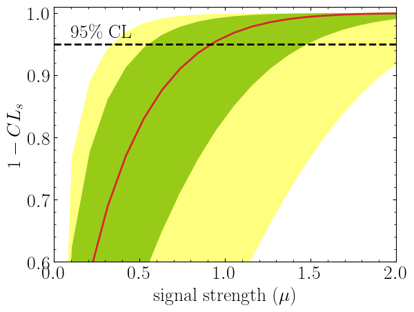
```python import matplotlib.pyplot as plt import numpy as np

poi = np.linspace(0,10,20) poiUL = np.array([statmodel.exclusionconfidencelevel(poitest=p, expected=spey.ExpectationType.aposteriori) for p in poi]) plt.plot(poi, poiUL[:,2], color="tab:red") plt.fillbetween(poi, poiUL[:,1], poiUL[:,3], alpha=0.8, color="green", lw=0) plt.fillbetween(poi, poiUL[:,0], poiUL[:,4], alpha=0.5, color="yellow", lw=0) plt.plot([0,10], [.95,.95], color="k", ls="dashed") plt.xlabel(r"${\rm signal\ strength}\ (\mu)$") plt.ylabel("$CL_s$") plt.xlim([0,10]) plt.ylim([0.6,1.01]) plt.text(0.5,0.96, r"$95\%\ {\rm CL}$") plt.show() ```

Here in the first line, we extract $CL_s$ values per POI for spey.ExpectationType.aposteriori expectation type, and we plot specific standard deviations, which provide the following plot:

The excluded value of POI can also be retrieved by spey.StatisticalModel.poiupperlimitfunction, which is the exact point where the red-curve and black dashed line meet. The upper limit for the $\pm1\sigma$ or $\pm2\sigma$ bands can be extracted by settingexpected_pvalueto"1sigma" or"2sigma"`` respectively, e.g.

```python statmodel.poiupperlimit(expected=spey.ExpectationType.aposteriori, expectedpvalue="1sigma")

[0.5507713378348318, 0.9195052042538805, 1.4812721449679866]

```

At a lower level, one can extract the likelihood information for the statistical model by calling spey.StatisticalModel.likelihood and spey.StatisticalModel.maximize_likelihood functions. By default, these will return negative log-likelihood values, but this can be changed via return_nll=False argument.

```python muhatobs, maxllhdobs = statmodel.maximizelikelihood(returnnll=False, ) muhatapri, maxllhdapri = statmodel.maximizelikelihood(returnnll=False, expected=spey.ExpectationType.apriori)

poi = np.linspace(-3,4,60)

llhdobs = np.array([statmodel.likelihood(p, returnnll=False) for p in poi]) llhdapri = np.array([statmodel.likelihood(p, expected=spey.ExpectationType.apriori, returnnll=False) for p in poi]) ```

Here, in the first two lines, we extracted the maximum likelihood and the POI value that maximizes the likelihood for two different expectation types. In the following, we computed likelihood distribution for various POI values, which then can be plotted as follows

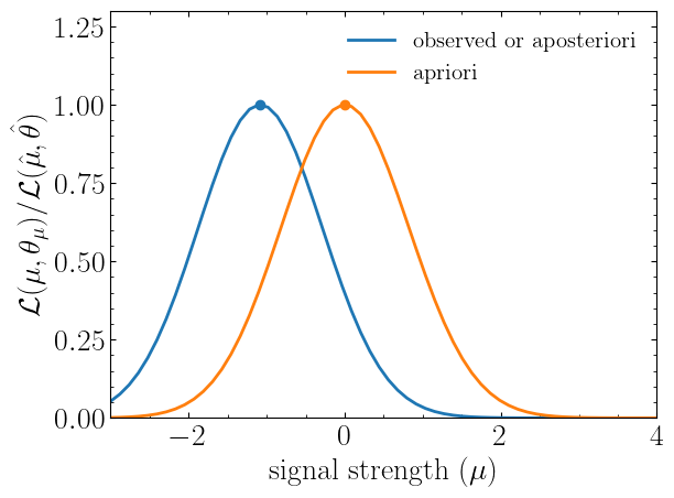
python plt.plot(poi, llhd_obs/maxllhd_obs, label=r"${\rm observed\ or\ aposteriori}$") plt.plot(poi, llhd_apri/maxllhd_apri, label=r"${\rm apriori}$") plt.scatter(muhat_obs, 1) plt.scatter(muhat_apri, 1) plt.legend(loc="upper right") plt.ylabel(r"$\mathcal{L}(\mu,\theta_\mu)/\mathcal{L}(\hat\mu,\hat\theta)$") plt.xlabel(r"${\rm signal\ strength}\ (\mu)$") plt.ylim([0,1.3]) plt.xlim([-3,4]) plt.show()

Notice the slight difference between likelihood distributions; this is because of the use of different expectation types. The dots on the likelihood distribution represent the point where the likelihood is maximized. Since for a spey.ExpectationType.apriori likelihood distribution observed and background values are the same, the likelihood should peak at $\mu=0$.