KerrGeoPy
KerrGeoPy: A Python Package for Computing Timelike Geodesics in Kerr Spacetime - Published in JOSS (2024)
Science Score: 100.0%
This score indicates how likely this project is to be science-related based on various indicators:
-
✓CITATION.cff file
Found CITATION.cff file -
✓codemeta.json file
Found codemeta.json file -
✓.zenodo.json file
Found .zenodo.json file -
✓DOI references
Found 10 DOI reference(s) in README and JOSS metadata -
✓Academic publication links
Links to: arxiv.org, joss.theoj.org, zenodo.org -
✓Committers with academic emails
1 of 2 committers (50.0%) from academic institutions -
○Institutional organization owner
-
✓JOSS paper metadata
Published in Journal of Open Source Software
Scientific Fields
Repository
Python library for computing properties of stable and plunging orbits around a spinning black hole
Basic Info
- Host: GitHub
- Owner: BlackHolePerturbationToolkit
- License: mit
- Language: Python
- Default Branch: main
- Homepage: https://kerrgeopy.readthedocs.io
- Size: 21.1 MB
Statistics
- Stars: 27
- Watchers: 6
- Forks: 4
- Open Issues: 1
- Releases: 4
Metadata Files
README.md

![]()


![]()

KerrGeoPy
KerrGeoPy is a python implementation of the KerrGeodesics Mathematica library. It is intended for use in computing orbital trajectories for extreme-mass-ratio inspirals (EMRIs). It implements the analytical solutions for plunging orbits from Dyson and van de Meent, as well as solutions for stable orbits from Fujita and Hikida. The library also provides a set of methods for computing constants of motion and orbital frequencies. See the documentation for more information.
Installation
Install using Anaconda
bash
conda install -c conda-forge kerrgeopy
or using pip
bash
pip install kerrgeopy
Note
This library uses functions introduced in scipy 1.8, so it may also be necessary to update scipy by running
pip install scipy -U, although in most cases this should be done automatically by pip. Certain plotting and animation functions also make use of features introduced in matplotlib 3.7 and rely on ffmpeg, which can be easily installed using homebrew or anaconda.
Contributing
For contribution guidelines, see CONTRIBUTING.
Stable Bound Orbits
KerrGeoPy computes orbits in Boyer-Lindquist coordinates $(t,r,\theta,\phi)$. Let $M$ to represent the mass of the primary body and let $J$ represent its angular momentum. Working in geometrized units where $G=c=1$, stable bound orbits are parametrized using the following variables:
$a$ - spin of the primary body
$p$ - orbital semilatus rectum
$e$ - orbital eccentricity
$x$ - cosine of the orbital inclination
$$ a = \frac{J}{M^2}, \quad\quad p = \frac{2r{\text{min}}r{\text{max}}}{M(r{\text{min}}+r{\text{max}})}, \quad\quad e = \frac{r{\text{max}}-r{\text{min}}}{r{\text{max}}+r{\text{min}}}, \quad\quad x = \cos{\theta_{\text{inc}}} $$
Note that $a$ and $x$ are restricted to values between -1 and 1, while $e$ is restricted to values between 0 and 1. Retrograde orbits are represented using a negative value for $a$ or for $x$. Polar orbits, marginally bound orbits, and orbits around an extreme Kerr black hole are not supported.
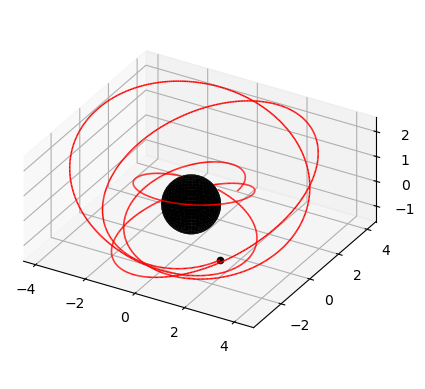
First, construct a StableOrbit using the four parameters described above.
```python import kerrgeopy as kg from math import cos, pi
orbit = kg.StableOrbit(0.999,3,0.4,cos(pi/6)) ```
Plot the orbit from $\lambda = 0$ to $\lambda = 10$ using the plot() method
python
fig, ax = orbit.plot(0,10)
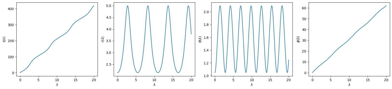
Next, compute the time, radial, polar and azimuthal components of the trajectory as a function of Mino time using the trajectory() method. By default, the time and radial components of the trajectory are given in geometrized units and are normalized using $M$ so that they are dimensionless.
python
t, r, theta, phi = orbit.trajectory()
```python import numpy as np import matplotlib.pyplot as plt
time = np.linspace(0,20,200)
plt.figure(figsize=(20,4))
plt.subplot(1,4,1) plt.plot(time, t(time)) plt.xlabel("$\lambda$") plt.ylabel(r"$t(\lambda)$")
plt.subplot(1,4,2) plt.plot(time, r(time)) plt.xlabel("$\lambda$") plt.ylabel("$r(\lambda)$")
plt.subplot(1,4,3) plt.plot(time, theta(time)) plt.xlabel("$\lambda$") plt.ylabel(r"$\theta(\lambda)$")
plt.subplot(1,4,4) plt.plot(time, phi(time)) plt.xlabel("$\lambda$") plt.ylabel(r"$\phi(\lambda)$") ```

Orbital Properties
Use the constants_of_motion() method to compute the dimensionless energy, angular momentum and Carter constant. By default, constants of motion are given in geometrized units where $G=c=1$ and are scale-invariant, meaning that they are normalized according to the masses of the two bodies as follows:
$$ \mathcal{E} = \frac{E}{\mu}, \quad \mathcal{L} = \frac{L}{\mu M}, \quad \mathcal{Q} = \frac{Q}{\mu^2 M^2} $$
Here, $M$ is the mass of the primary body and $\mu$ is the mass of the secondary body.
Frequencies of motion can be computed in Mino time using the mino_frequencies() method and in Boyer-Lindquist time using the fundamental_frequencies() method. As with constants of motion, the frequencies returned by both methods are given in geometrized units and are normalized by $M$ so that they are dimensionless.
```python from IPython.display import display, Math
E, L, Q = orbit.constantsofmotion()
upsilonr, upsilontheta, upsilonphi, gamma = orbit.minofrequencies()
omegar, omegatheta, omegaphi = orbit.fundamentalfrequencies()
display(Math(fr"a = {orbit.a} \quad p = {orbit.p} \quad e = {orbit.e} \quad x = {orbit.x}"))
display(Math(fr"\mathcal{{E}} = {E:.3f} \quad \mathcal{{L}} = {L:.3f} \quad \mathcal{{Q}} = {Q:.3f}"))
display(Math(fr"""\Upsilonr = {upsilonr:.3f} \quad \Upsilon\theta = {upsilontheta:.3f} \quad \Upsilon\phi = {upsilonphi:.3f} \quad \Gamma = {gamma:.3f}"""))
display(Math(fr"""\Omegar = {omegar:.3f} \quad \Omega\theta = {omegatheta:.3f} \quad \Omega\phi = {omegaphi:.3f}""")) ```
$\displaystyle a = 0.999 \quad p = 3 \quad e = 0.4 \quad x = 0.8660254037844387$
$\displaystyle \mathcal{E} = 0.877 \quad \mathcal{L} = 1.903 \quad \mathcal{Q} = 1.265$
$\displaystyle \Upsilonr = 1.145 \quad \Upsilon\theta = 2.243 \quad \Upsilon_\phi = 3.118 \quad \Gamma = 20.531$
$\displaystyle \Omegar = 0.056 \quad \Omega\theta = 0.109 \quad \Omega_\phi = 0.152$
Plunging Orbits
Plunging orbits are parametrized using the spin parameter and the three constants of motion.
$a$ - spin of the primary body
$\mathcal{E}$ - Energy
$\mathcal{L}$ - $z$-component of angular momentum
$\mathcal{Q}$ - Carter constant
It is assumed that all orbital parameters are given in geometrized units where $G=c=1$ and are normalized according to the masses of the two bodies as follows:
$$ a = \frac{J}{M^2}, \quad \mathcal{E} = \frac{E}{\mu}, \quad \mathcal{L} = \frac{L}{\mu M}, \quad \mathcal{Q} = \frac{Q}{\mu^2 M^2} $$
Construct a PlungingOrbit by passing in these four parameters.
python
orbit = kg.PlungingOrbit(0.9, 0.94, 0.1, 12)
As with stable orbits, the components of the trajectory can be computed using the trajectory() method
python
t, r, theta, phi = orbit.trajectory()
```python import numpy as np import matplotlib.pyplot as plt
time = np.linspace(0,20,200)
plt.figure(figsize=(20,4))
plt.subplot(1,4,1) plt.plot(time, t(time)) plt.xlabel("$\lambda$") plt.ylabel(r"$t(\lambda)$")
plt.subplot(1,4,2) plt.plot(time, r(time)) plt.xlabel("$\lambda$") plt.ylabel("$r(\lambda)$")
plt.subplot(1,4,3) plt.plot(time, theta(time)) plt.xlabel("$\lambda$") plt.ylabel(r"$\theta(\lambda)$")
plt.subplot(1,4,4) plt.plot(time, phi(time)) plt.xlabel("$\lambda$") plt.ylabel(r"$\phi(\lambda)$") ```

Alternative Parametrizations
Use the from_constants() class method to construct a StableOrbit from the spin parameter and constants of motion $(a,E,L,Q)$
python
orbit = kg.StableOrbit.from_constants(0.9, 0.95, 1.6, 8)
Use the Orbit class to construct an orbit from the spin parameter $a$, initial position $(t0,r0,\theta0,\phi0)$ and initial four-velocity $(u^t0,u^r0,u^{\theta}0,u^{\phi}0)$
```python stable_orbit = kg.StableOrbit(0.999,3,0.4,cos(pi/6))
x0 = stableorbit.initialposition u0 = stableorbit.initialvelocity
orbit = kg.Orbit(0.999,x0,u0) ```
```python t, r, theta, phi = orbit.trajectory()
time = np.linspace(0,20,200)
plt.figure(figsize=(20,4))
plt.subplot(1,4,1) plt.plot(time, t(time)) plt.xlabel("$\lambda$") plt.ylabel(r"$t(\lambda)$")
plt.subplot(1,4,2) plt.plot(time, r(time)) plt.xlabel("$\lambda$") plt.ylabel("$r(\lambda)$")
plt.subplot(1,4,3) plt.plot(time, theta(time)) plt.xlabel("$\lambda$") plt.ylabel(r"$\theta(\lambda)$")
plt.subplot(1,4,4) plt.plot(time, phi(time)) plt.xlabel("$\lambda$") plt.ylabel(r"$\phi(\lambda)$") ```
Citation
If you use this software, please cite our article in the Journal of Open Source Software.
@article{kerrgeopy,
doi = {10.21105/joss.06587},
url = {https://doi.org/10.21105/joss.06587},
year = {2024},
publisher = {The Open Journal},
volume = {9},
number = {98},
pages = {6587},
author = {Seyong Park and Zachary Nasipak},
title = {KerrGeoPy: A Python Package for Computing Timelike Geodesics in Kerr Spacetime},
journal = {Journal of Open Source Software}
}
Authors
- Seyong Park
- Zach Nasipak
Owner
- Name: Black Hole Perturbation Toolkit
- Login: BlackHolePerturbationToolkit
- Kind: organization
- Website: bhptoolkit.org
- Repositories: 14
- Profile: https://github.com/BlackHolePerturbationToolkit
Open tools for black hole perturbation theory
JOSS Publication
KerrGeoPy: A Python Package for Computing Timelike Geodesics in Kerr Spacetime
Authors

NASA Goddard Space Flight Center, Greenbelt, MD, USA, University of Maryland, College Park, MD, USA
NASA Goddard Space Flight Center, Greenbelt, MD, USA
Editor
Juanjo Bazán
Tags
black holes perturbation theory gravitational wavesCitation (CITATION.cff)
cff-version: "1.2.0"
authors:
- family-names: Park
  given-names: Seyong
  orcid: "https://orcid.org/0009-0002-1152-9324"
- family-names: Nasipak
  given-names: Zachary
  orcid: "https://orcid.org/0000-0002-5109-9704"
doi: 10.5281/zenodo.11386563
message: If you use this software, please cite our article in the
  Journal of Open Source Software.
preferred-citation:
  authors:
  - family-names: Park
    given-names: Seyong
    orcid: "https://orcid.org/0009-0002-1152-9324"
  - family-names: Nasipak
    given-names: Zachary
    orcid: "https://orcid.org/0000-0002-5109-9704"
  date-published: 2024-06-01
  doi: 10.21105/joss.06587
  issn: 2475-9066
  issue: 98
  journal: Journal of Open Source Software
  publisher:
    name: Open Journals
  start: 6587
  title: "KerrGeoPy: A Python Package for Computing Timelike Geodesics
    in Kerr Spacetime"
  type: article
  url: "https://joss.theoj.org/papers/10.21105/joss.06587"
  volume: 9
title: "`KerrGeoPy`: A Python Package for Computing Timelike Geodesics
  in Kerr Spacetime"
GitHub Events
Total
- Issues event: 2
- Watch event: 3
- Issue comment event: 1
- Pull request event: 1
- Fork event: 2
Last Year
- Issues event: 2
- Watch event: 3
- Issue comment event: 1
- Pull request event: 1
- Fork event: 2
Committers
Last synced: 12 months ago
Top Committers
| Name | Commits | |
|---|---|---|
| Se Yong Park | s****1@g****m | 145 |
| Se Yong Park | s****9@g****v | 3 |
Committer Domains (Top 20 + Academic)
Issues and Pull Requests
Last synced: 11 months ago
All Time
- Total issues: 3
- Total pull requests: 11
- Average time to close issues: 2 months
- Average time to close pull requests: 3 days
- Total issue authors: 3
- Total pull request authors: 4
- Average comments per issue: 1.33
- Average comments per pull request: 0.18
- Merged pull requests: 9
- Bot issues: 0
- Bot pull requests: 0
Past Year
- Issues: 1
- Pull requests: 2
- Average time to close issues: 28 minutes
- Average time to close pull requests: N/A
- Issue authors: 1
- Pull request authors: 1
- Average comments per issue: 1.0
- Average comments per pull request: 0.5
- Merged pull requests: 0
- Bot issues: 0
- Bot pull requests: 0
Top Authors
Issue Authors
- AnujKankani (1)
- znasipak (1)
- nielsw2 (1)
Pull Request Authors
- syp2001 (11)
- TVTien83 (2)
- xuanxu (2)
- dfm (2)
Top Labels
Issue Labels
Pull Request Labels
Packages
- Total packages: 1
-
Total downloads:
- pypi 25 last-month
- Total dependent packages: 0
- Total dependent repositories: 0
- Total versions: 9
- Total maintainers: 1
pypi.org: kerrgeopy
Library for computing stable and plunging geodesics in Kerr spacetime
- Homepage: https://github.com/BlackHolePerturbationToolkit/KerrGeoPy
- Documentation: https://kerrgeopy.readthedocs.io/
- License: MIT License
-
Latest release: 0.9.3
published about 2 years ago
Rankings
Maintainers (1)
Dependencies
- scipy *
- actions/checkout v3 composite
- actions/setup-python v3 composite
- pypa/gh-action-pypi-publish 27b31702a0e7fc50959f5ad993c78deac1bdfc29 composite
- actions/checkout v3 composite
- actions/setup-python v3 composite