oceanmesh
Automatic coastal ocean mesh generation in Python and C++. **under development**
Science Score: 49.0%
This score indicates how likely this project is to be science-related based on various indicators:
-
○CITATION.cff file
-
✓codemeta.json file
Found codemeta.json file -
✓.zenodo.json file
Found .zenodo.json file -
✓DOI references
Found 3 DOI reference(s) in README -
✓Academic publication links
Links to: sciencedirect.com, springer.com -
○Committers with academic emails
-
○Institutional organization owner
-
○JOSS paper metadata
-
○Scientific vocabulary similarity
Low similarity (15.2%) to scientific vocabulary
Keywords
Keywords from Contributors
Repository
Automatic coastal ocean mesh generation in Python and C++. **under development**
Basic Info
Statistics
- Stars: 63
- Watchers: 15
- Forks: 22
- Open Issues: 20
- Releases: 3
Topics
Metadata Files
README.md
oceanmesh: Automatic coastal ocean mesh generation
:ocean: :cyclone:
![]()
![]()
Coastal ocean mesh generation from vector and raster GIS data.
Table of contents
- oceanmesh
- Table of contents
- Functionality
- Citing
- Questions or problems
- Installation
- Examples
- Testing
- License <!--te-->
Functionality
- A Python package for the development of unstructured triangular meshes that are used in the simulation of coastal ocean circulation. The software integrates mesh generation directly with geophysical datasets such as topo-bathymetric rasters/digital elevation models and shapefiles representing coastal features. It provides some necessary pre- and post-processing tools to inevitably perform a successful numerical simulation with the developed model.
- Automatically deal with arbitrarily complex shoreline vector datasets that represent complex coastal boundaries and incorporate the data in an automatic-sense into the mesh generation process.
- A variety of commonly used mesh size functions to distribute element sizes that can easily be controlled via a simple scripting application interface.
- Mesh checking and clean-up methods to avoid simulation problems.
Citing
The Python version of the algorithm does not yet have a citation; however, similar algorithms and ideas are shared between both version.
[1] - Roberts, K. J., Pringle, W. J., and Westerink, J. J., 2019.
      OceanMesh2D 1.0: MATLAB-based software for two-dimensional unstructured mesh generation in coastal ocean modeling,
      Geoscientific Model Development, 12, 1847-1868. https://doi.org/10.5194/gmd-12-1847-2019.
Questions or problems
Besides posting issues with the code on Github, you can also ask questions via our Slack channel here.
Otherwise please reach out to Dr. Keith Roberts (keithrbt0@gmail.com) with questions or concerns!
Please include version information when posting bug reports.
oceanmesh uses versioneer.
The version can be inspected through Python
python -c "import oceanmesh; print(oceanmesh.__version__)"
or through
python setup.py version
in the working directory.
To see what's going on with oceanmesh when running scripts, you can turn on logging (which is by default suppressed) by importing the two modules sys and logging and then placing one of the three following logging commands after your imports in your calling script. The amount of information returned is the greatest with logging.DEBUG and leas with logging.WARNING.
```
import logging
import sys
logging.basicConfig(stream=sys.stdout, level=logging.WARNING)
logging.basicConfig(stream=sys.stdout, level=logging.INFO)
logging.basicConfig(stream=sys.stdout, level=logging.DEBUG)
```
Installation
The notes below refer to installation on platforms other than MS Windows. For Windows, refer to the following section.
For installation, oceanmesh needs cmake, CGAL:
sudo apt install cmake libcgal-dev
CGAL and can also be installed with conda:
conda install -c conda-forge cgal
After that, clone the repo and oceanmesh can be updated/installed using pip.
pip install -U -e .
On some clusters/HPC in order to install CGAL, you may need to load/install gmp and mpfr. For example, to install:
sudo apt install libmpfr-dev libgmp3-dev
Installation on Windows
Python under Windows can easily experience DLL hell due to version incompatibilities. Such is the case for the combination of support packages required for OceanMesh. For this reason, we have provided 'install_cgal.bat' to build a CGAL development distribution separately as a prerequisite.
Prerequisites to build CGAL using the provided batch file are as follows:
- Windows 10 or later
- Visual Studio with C++
- CMake
- Git
After successful intallation of a CGAL development package, proceed via one of the two options below to generate a python environment with OceanMesh installed.
If you are using a conda-based Python distribution, then 'install_oceanmesh.bat' should take care of everything, provided no package conflicts arise.
If you have a different Python distribution, or if you do not want to use packages from conda forge, then the following process may be required:
- Obtain binary wheels for your python distribution for the latest GDAL, Fiona, and Rasterio (https://www.lfd.uci.edu/~gohlke/pythonlibs).
- Create a new virtual environment and activate it.
- Execute: cmd.exe /C "for %f in (GDAL*.whl Fiona*.whl rasterio*.whl) do pip install %f"
- Execute: pip install geopandas rasterio scikit-fmm pybind11
- Execute: python setup.py install
:warning:
WARNING: THIS PROGRAM IS IN ACTIVE DEVELOPMENT. INSTALLATION IS ONLY RECOMMENDED FOR DEVELOPERS AT THIS TIME. WHEN A STABLE API IS REACHED, THE PROGRAM WILL BE AVAILABLE VIA pypi
Examples
Setting the region
oceanmesh can mesh a polygonal region in the vast majority of coordinate reference systems (CRS). Thus, all oceanmesh scripts begin with declaring the extent and CRS to be used and/or transofmring to a different CRS like this.
```python import oceanmesh as om
EPSG = 32619 # A Python int, dict, or str containing the CRS information (in this case UTM19N) bbox = ( -70.29637, -43.56508, -69.65537, 43.88338, ) # the extent of the domain (can also be a multi-polygon delimited by rows of np.nan) extent = om.Region( extent=bbox, crs=4326 ) # set the region (the bbox is given here in EPSG:4326 or WGS84) extent = extent.transform_to(EPSG) # Now I transform to the desired EPSG (UTM19N) print( extent.bbox ) # now the extents are in the desired CRS and can be passed to various functions later on ```
Reading in geophysical data
oceanmesh uses shoreline vector datasets (i.e., ESRI shapefiles) and digital elevation models (DEMs) to construct mesh size functions and signed distance functions to adapt mesh resolution for complex and irregularly shaped coastal ocean domains.
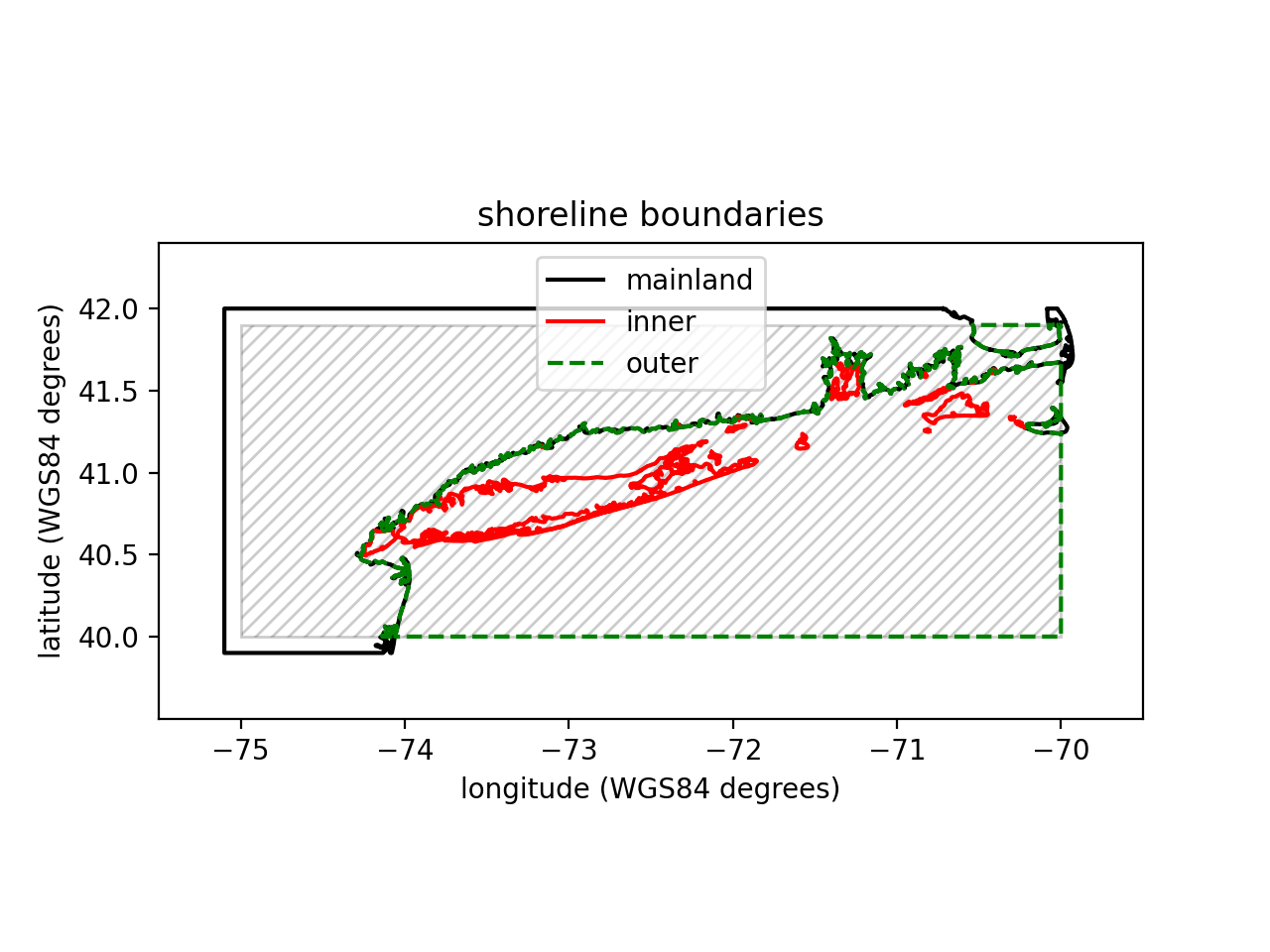
Shoreline datasets are necessary to build signed distance functions which define the meshing domain. Here we show how to download a world shoreline dataset referred to as GSHHG and read it into to oceanmesh.
```python import zipfile
import requests
import oceanmesh as om
Download and load the GSHHS shoreline
url = "http://www.soest.hawaii.edu/pwessel/gshhg/gshhg-shp-2.3.7.zip" filename = url.split("/")[-1] with open(filename, "wb") as f: r = requests.get(url) f.write(r.content)
with zipfile.ZipFile("gshhg-shp-2.3.7.zip", "r") as zipref: zipref.extractall("gshhg-shp-2.3.7")
fname = "gshhg-shp-2.3.7/GSHHSshp/f/GSHHSf_L1.shp" EPSG = 4326 # EPSG code for WGS84 which is what you want to mesh in
Specify and extent to read in and a minimum mesh size in the unit of the projection
extent = om.Region(extent=(-75.000, -70.001, 40.0001, 41.9000), crs=EPSG) minedgelength = 0.01 # In the units of the projection! shoreline = om.Shoreline( fname, extent.bbox, minedgelength, crs=EPSG ) # NB: the Shoreline class assumes WGS84:4326 if not specified shoreline.plot( xlabel="longitude (WGS84 degrees)", ylabel="latitude (WGS84 degrees)", title="shoreline boundaries", )
Using our shoreline, we create a signed distance function
which will be used for meshing later on.
sdf = om.signeddistancefunction(shoreline)
```
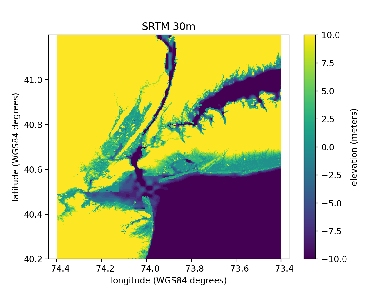
DEMs are used to build some mesh size functions (e.g., wavelength, enforcing size bounds, enforce maximum Courant bounds) but are not essential for mesh generation purposes. The DEM used below 'Eastcoast.nc' was created using the Python package elevation with the following command:
<!--pytest-codeblocks:skip-->
eio clip - o EastCoast.nc --bounds -74.4 40.2 -73.4 41.2
This data is a clip from the SRTM30 m elevation dataset.
```python import oceanmesh as om
fdem = "datasets/EastCoast.nc"
Digital Elevation Models (DEM) can be read into oceanmesh in
either the NetCDF format or GeoTiff format provided they are
in geographic coordinates (WGS84)
If no extents are passed (i.e., the kwarg bbox), then the entire extent of the
DEM is read into memory.
Note: the DEM will be projected to the desired CRS automatically.
EPSG = 4326
dem = om.DEM(fdem, crs=EPSG)
dem.plot(
xlabel="longitude (WGS84 degrees)",
ylabel="latitude (WGS84 degrees)",
title="SRTM 30m",
cbarlabel="elevation (meters)",
vmin=-10, # minimum elevation value in plot
vmax=10, # maximum elevation value in plot
)
```
Defining the domain
The domain is defined by a signed distance function. A signed distance function can be automatically generated from a complex coastal ocean domain as such
```python import oceanmesh as om
fname = "gshhg-shp-2.3.7/GSHHSshp/f/GSHHSfL1.shp" EPSG = 4326 # EPSG:4326 or WGS84 extent = om.Region(extent=(-75.00, -70.001, 40.0001, 41.9000), crs=EPSG) minedgelength = 0.01 # minimum mesh size in domain in projection shoreline = om.Shoreline(fname, extent.bbox, minedge_length)
build a signed distance functiona automatically
sdf = om.signeddistancefunction(shoreline)
``
In some situations, it is necessary to flip the definition of what'sinsidethe meshing domain. This can be accomplished via theinvertkwarg for thesigneddistancefunction`.
python
sdf = om.signed_distance_function(shoreline, invert=True)
Setting invert=True will be mesh the 'land side' of the domain rather than the ocean.
Building mesh sizing functions
In oceanmesh mesh resolution can be controlled according to a variety of feature-driven geometric and topo-bathymetric functions. In this section, we briefly explain the major functions and present examples and code. Reasonable values for some of these mesh sizing functions and their affect on the numerical simulation of barotropic tides was investigated in Roberts et. al, 2019
All mesh size functions are defined on regular Cartesian grids. The properties of these grids are abstracted by the Grid class.
Distance and feature size
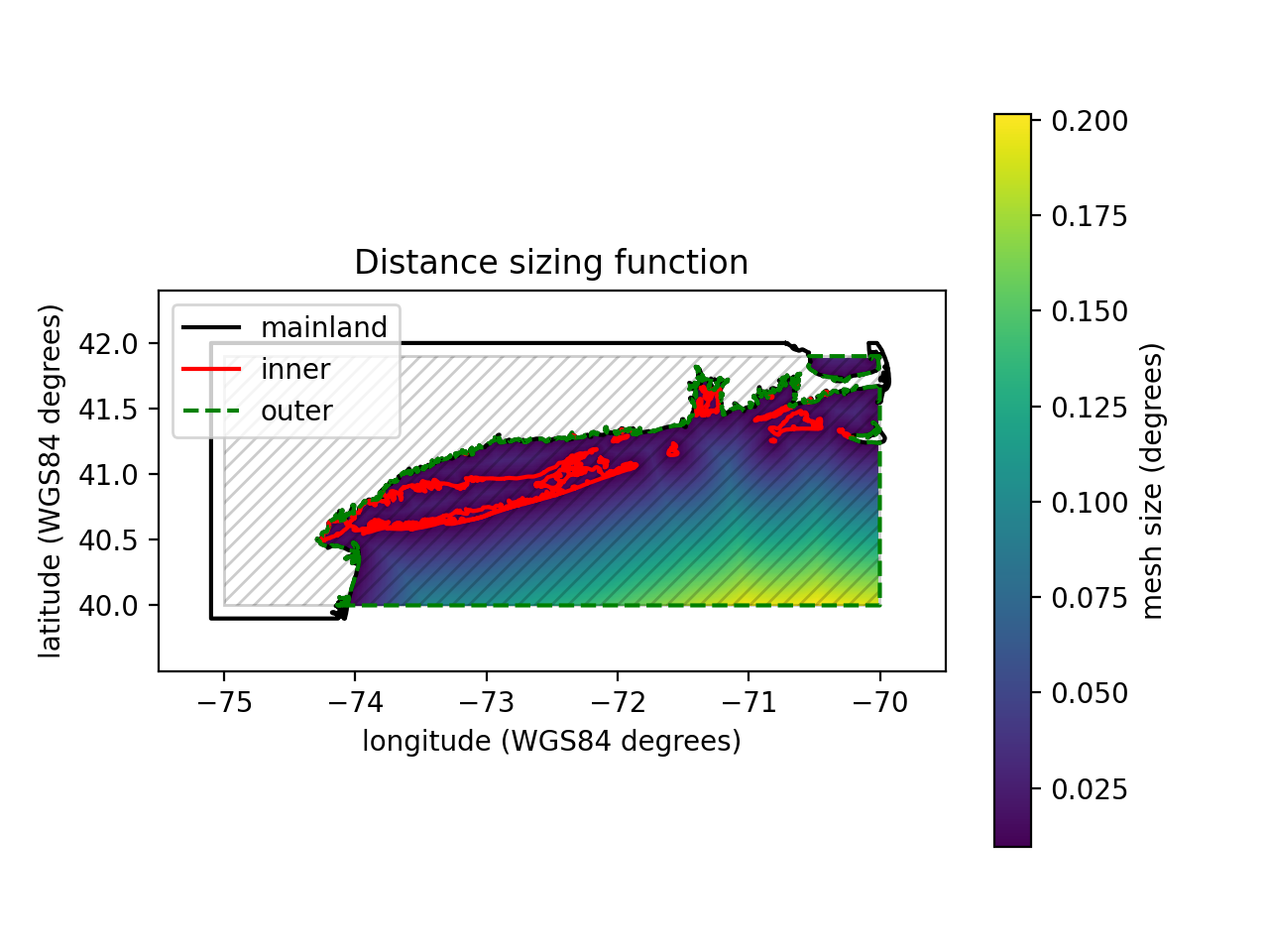
A high degree of mesh refinement is often necessary near the shoreline boundary to capture its geometric complexity. If mesh resolution is poorly distributed, critical conveyances may be missed, leading to larger-scale errors in the nearshore circulation. Thus, a mesh size function that is equal to a user-defined minimum mesh size h0 along the shoreline boundary, growing as a linear function of the signed distance d from it, may be appropriate.
```python import oceanmesh as om
fname = "gshhg-shp-2.3.7/GSHHSshp/f/GSHHSfL1.shp"
EPSG = 4326 # EPSG:4326 or WGS84
extent = om.Region(extent=(-75.00, -70.001, 40.0001, 41.9000), crs=EPSG)
minedgelength = 0.01 # minimum mesh size in domain in projection
shoreline = om.Shoreline(fname, extent.bbox, minedgelength)
edgelength = om.distancesizingfunction(shoreline, rate=0.15)
fig, ax, pc = edge_length.plot(
xlabel="longitude (WGS84 degrees)",
ylabel="latitude (WGS84 degrees)",
title="Distance sizing function",
cbarlabel="mesh size (degrees)",
holding=True,
)
shoreline.plot(ax=ax)
```
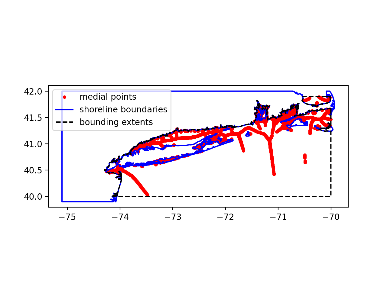
One major drawback of the distance mesh size function is that the minimum mesh size will be placed evenly along straight stretches of shoreline. If the distance mesh size function generates too many vertices (or your application can tolerate it), a feature mesh size function that places resolution according to the geometric width of the shoreline should be employed instead (Conroy et al., 2012;Koko, 2015).
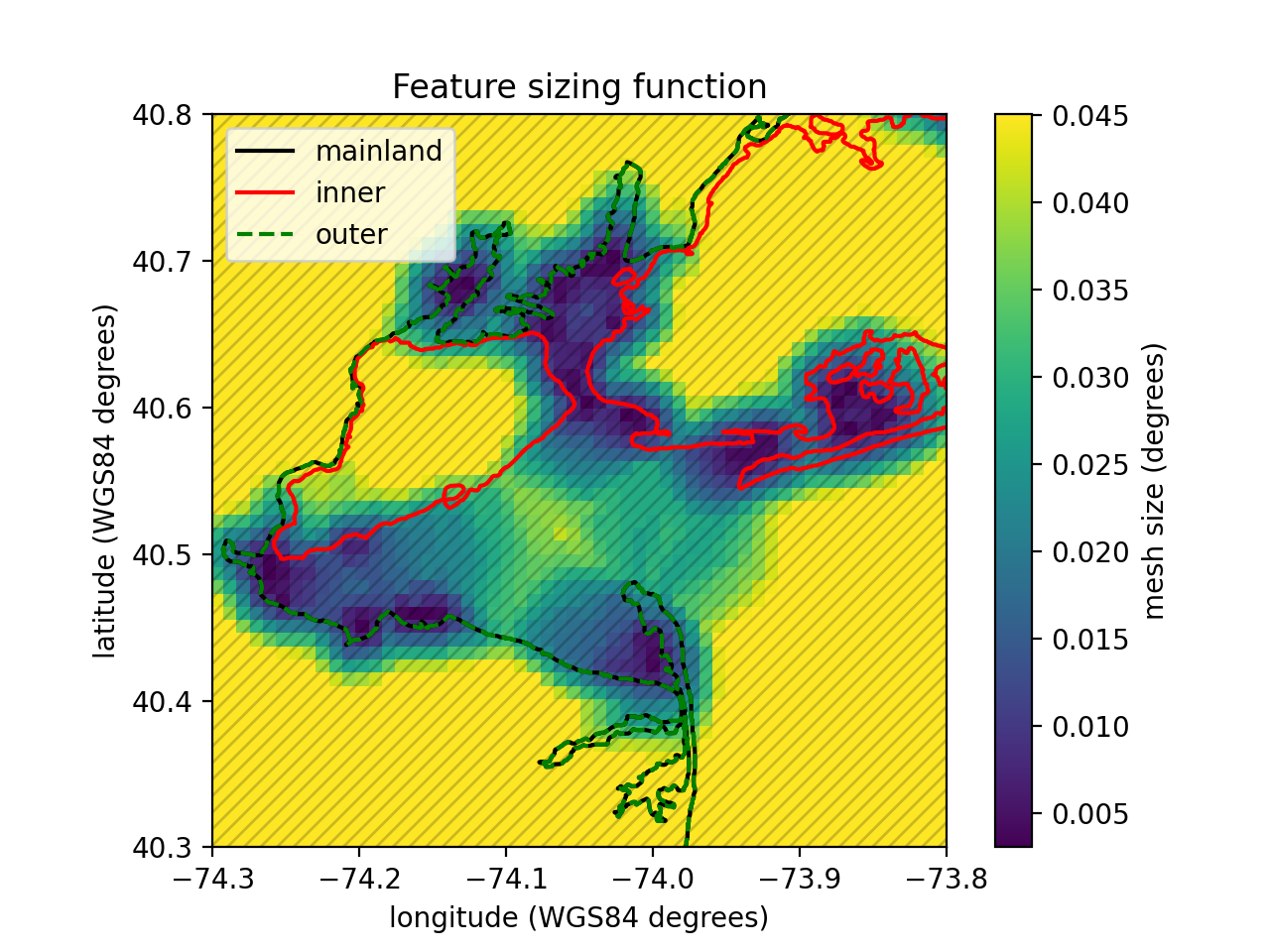
In this function, the feature size (e.g., the width of channels and/or tributaries and the radius of curvature of the shoreline) along the coast is estimated by computing distances to the medial axis of the shoreline geometry. In oceanmesh, we have implemented an approximate medial axis method closely following Koko, (2015).
```python import oceanmesh as om
fname = "gshhg-shp-2.3.7/GSHHSshp/f/GSHHSfL1.shp" EPSG = 4326 # EPSG:4326 or WGS84 extent = om.Region(extent=(-75.00, -70.001, 40.0001, 41.9000), crs=EPSG) minedgelength = 0.01 # minimum mesh size in domain in projection shoreline = om.Shoreline(fname, extent.bbox, minedgelength) sdf = om.signeddistance_function(shoreline)
Visualize the medial points
edgelength = om.featuresizingfunction(
shoreline, sdf, maxedgelength=0.05, plot=True
)
fig, ax, pc = edgelength.plot(
xlabel="longitude (WGS84 degrees)",
ylabel="latitude (WGS84 degrees)",
title="Feature sizing function",
cbarlabel="mesh size (degrees)",
holding=True,
xlim=[-74.3, -73.8],
ylim=[40.3, 40.8],
)
shoreline.plot(ax=ax)
```
Enforcing mesh size gradation
Some mesh size functions will not produce smooth element size transitions when meshed and this can lead to problems with numerical simulation. All mesh size function can thus be graded such that neighboring mesh sizes are bounded above by a constant. Mesh grading edits coarser regions and preserves the finer mesh resolution zones.
Repeating the above but applying a gradation rate of 15% produces the following: ```python import oceanmesh as om
fname = "gshhg-shp-2.3.7/GSHHSshp/f/GSHHSfL1.shp"
EPSG = 4326 # EPSG:4326 or WGS84
extent = om.Region(extent=(-75.00, -70.001, 40.0001, 41.9000), crs=EPSG)
minedgelength = 0.01 # minimum mesh size in domain in projection
shoreline = om.Shoreline(fname, extent.bbox, minedgelength)
sdf = om.signeddistancefunction(shoreline)
edgelength = om.featuresizingfunction(shoreline, sdf, maxedgelength=0.05)
edgelength = om.enforcemeshgradation(edgelength, gradation=0.15)
fig, ax, pc = edge_length.plot(
xlabel="longitude (WGS84 degrees)",
ylabel="latitude (WGS84 degrees)",
title="Feature sizing function with gradation bound",
cbarlabel="mesh size (degrees)",
holding=True,
xlim=[-74.3, -73.8],
ylim=[40.3, 40.8],
)
shoreline.plot(ax=ax)
```
Wavelength-to-gridscale
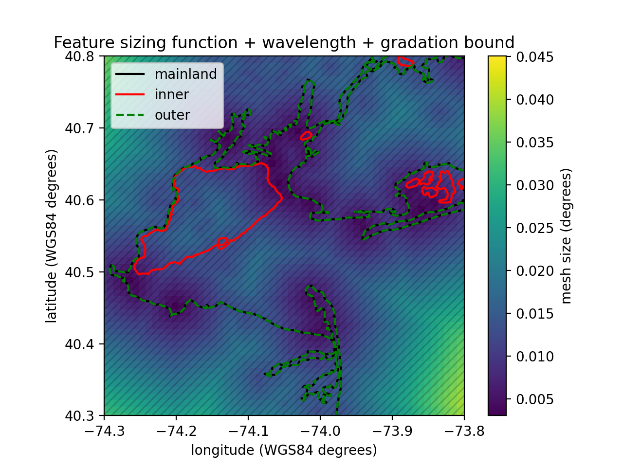
In shallow water theory, the wave celerity, and hence the wavelength λ, is proportional to the square root of the depth of the water column. This relationship indicates that more mesh resolution at shallower depths is required to resolve waves that are shorter than those in deep water. With this considered, a mesh size function hwl that ensures a certain number of elements are present per wavelength (usually of the M2-dominant semi-diurnal tidal species but the frequency of the dominant wave can be specified via kwargs) can be deduced.
In this snippet, as before we compute the feature size function, but now we also compute the wavelength-to-gridscale sizing function using the SRTM dataset and compute the minimum of all the functions before grading. We discretize the wavelength of the M2 by 30 elements (e.g., wl=30) ```python import oceanmesh as om
fdem = "datasets/EastCoast.nc" fname = "gshhg-shp-2.3.7/GSHHSshp/f/GSHHSf_L1.shp"
minedgelength = 0.01
extent = om.Region(extent=(-74.3, -73.8, 40.3,40.8), crs=4326) dem = om.DEM(fdem, bbox=extent,crs=4326) shoreline = om.Shoreline(fname, dem.bbox, minedgelength) sdf = om.signeddistancefunction(shoreline) edgelength1 = om.featuresizingfunction(shoreline, sdf, maxedgelength=0.05) edgelength2 = om.wavelengthsizingfunction( dem, wl=100, period=12.42 * 3600 ) # use the M2-tide period (in seconds)
Compute the minimum of the sizing functions
edgelength = om.computeminimum([edgelength1, edgelength2])
edgelength = om.enforcemeshgradation(edgelength, gradation=0.15)
fig, ax, pc = edge_length.plot(
xlabel="longitude (WGS84 degrees)",
ylabel="latitude (WGS84 degrees)",
title="Feature sizing function + wavelength + gradation bound",
cbarlabel="mesh size (degrees)",
holding=True,
xlim=[-74.3, -73.8],
ylim=[40.3, 40.8],
)
shoreline.plot(ax=ax)
```
Resolving bathymetric gradients
The distance, feature size, and/or wavelength mesh size functions can lead to coarse mesh resolution in deeper waters that under-resolve and smooth over the sharp topographic gradients that characterize the continental shelf break. These slope features can be important for coastal ocean models in order to capture dissipative effects driven by the internal tides, transmissional reflection at the shelf break that controls the astronomical tides, and trapped shelf waves. The bathymetry field contains often excessive details that are not relevant for most flows, thus the bathymetry can be smoothed by a variety of filters (e.g., lowpass, bandpass, and highpass filters) before calculating the mesh sizes.
```python import oceanmesh as om
fdem = "datasets/EastCoast.nc" fname = "gshhg-shp-2.3.7/GSHHSshp/f/GSHHSf_L1.shp"
EPSG = 4326 # EPSG:4326 or WGS84 bbox = (-74.4, -73.4, 40.2, 41.2) extent = om.Region(extent=bbox, crs=EPSG) dem = om.DEM(fdem, crs=EPSG)
minedgelength = 0.0025 # minimum mesh size in domain in projection maxedgelength = 0.10 # maximum mesh size in domain in projection shoreline = om.Shoreline(fname, extent.bbox, minedgelength) sdf = om.signeddistancefunction(shoreline)
edgelength1 = om.featuresizingfunction( shoreline, sdf, maxedgelength=maxedgelength, crs=EPSG, ) edgelength2 = om.bathymetricgradientsizingfunction( dem, slopeparameter=5.0, filterquotient=50, minedgelength=minedgelength, maxedgelength=maxedgelength, crs=EPSG, ) # will be reactivated edgelength3 = om.computeminimum([edgelength1, edgelength2]) edgelength3 = om.enforcemeshgradation(edge_length3, gradation=0.15) ```
Cleaning up the mesh
After mesh generation has terminated, a secondary round of mesh improvement strategies is applied that is focused towards improving the geometrically worst-quality triangles that often occur near the boundary of the mesh and can make simulation impossible. Low-quality triangles can occur near the mesh boundary because the geospatial datasets used may contain features that have horizontal length scales smaller than the minimum mesh resolution. To handle this issue, a set of algorithms is applied that iteratively addresses the vertex connectivity problems. The application of the following mesh improvement strategies results in a simplified mesh boundary that conforms to the user-requested minimum element size.
Topological defects in the mesh can be removed by ensuring that it is valid, defined as having the following properties:
the vertices of each triangle are arranged in counterclockwise order;
conformity (a triangle is not allowed to have a vertex of another triangle in its interior); and
traversability (the number of boundary segments is equal to the number of boundary vertices, which guarantees a unique path along the mesh boundary).
Here are some of the relevant codes to address these common problems. <!--pytest-codeblocks:skip--> ```python
Address (1) above.
points, cells = fix_mesh(points, cells)
Addresses (2)-(3) above. Remove degenerate mesh faces and other common problems in the mesh
points, cells = makemeshboundaries_traversable(points, cells)
Remove elements (i.e., "faces") connected to only one channel
These typically occur in channels at or near the grid scale.
points, cells = deletefacesconnectedtoone_face(points, cells)
Remove low quality boundary elements less than min_qual
points, cells = deleteboundaryfaces(points, cells, min_qual=0.15)
Apply a Laplacian smoother that preserves the element density
points, cells = laplacian2(points, cells) ```
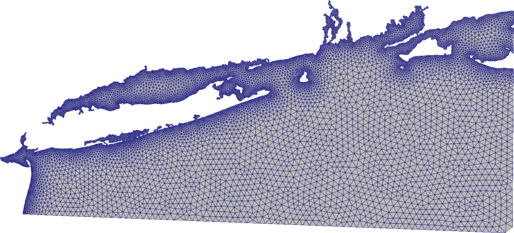
Mesh generation
Mesh generation is based on the DistMesh algorithm and requires only a signed distance function and a mesh sizing function. These two functions can be defined through the previously elaborated commands above; however, they can also be straightforward functions that take an array of point coordinates and return the signed distance/desired mesh size.
In this example, we demonstrate all of the above to build a mesh around New York, United States with an approximate minimum element size of around 1 km expanding linear with distance from the shoreline to an approximate maximum element size of 5 km.
Here we use the GSHHS shoreline here and the Python package meshio to write the mesh to a VTK file for visualization in ParaView. Other mesh formats are possible; see meshio for more details
```python import meshio import oceanmesh as om
fname = "gshhg-shp-2.3.7/GSHHSshp/f/GSHHSf_L1.shp"
EPSG = 4326 # EPSG:4326 otherwise known as WGS84 extent = om.Region(extent=(-75.00, -70.001, 40.0001, 41.9000), crs=EPSG) minedgelength = 0.01 # minimum mesh size in domain in projection
shore = om.Shoreline(fname, extent.bbox, minedgelength)
edgelength = om.distancesizingfunction(shore, maxedge_length=0.05)
domain = om.signeddistancefunction(shore)
points, cells = om.generatemesh(domain, edgelength)
remove degenerate mesh faces and other common problems in the mesh
points, cells = om.makemeshboundaries_traversable(points, cells)
points, cells = om.deletefacesconnectedtoone_face(points, cells)
remove low quality boundary elements less than 15%
points, cells = om.deleteboundaryfaces(points, cells, min_qual=0.15)
apply a Laplacian smoother
points, cells = om.laplacian2(points, cells)
write the mesh with meshio
meshio.writepointscells( "newyork.vtk", points, [("triangle", cells)], fileformat="vtk", ) ```
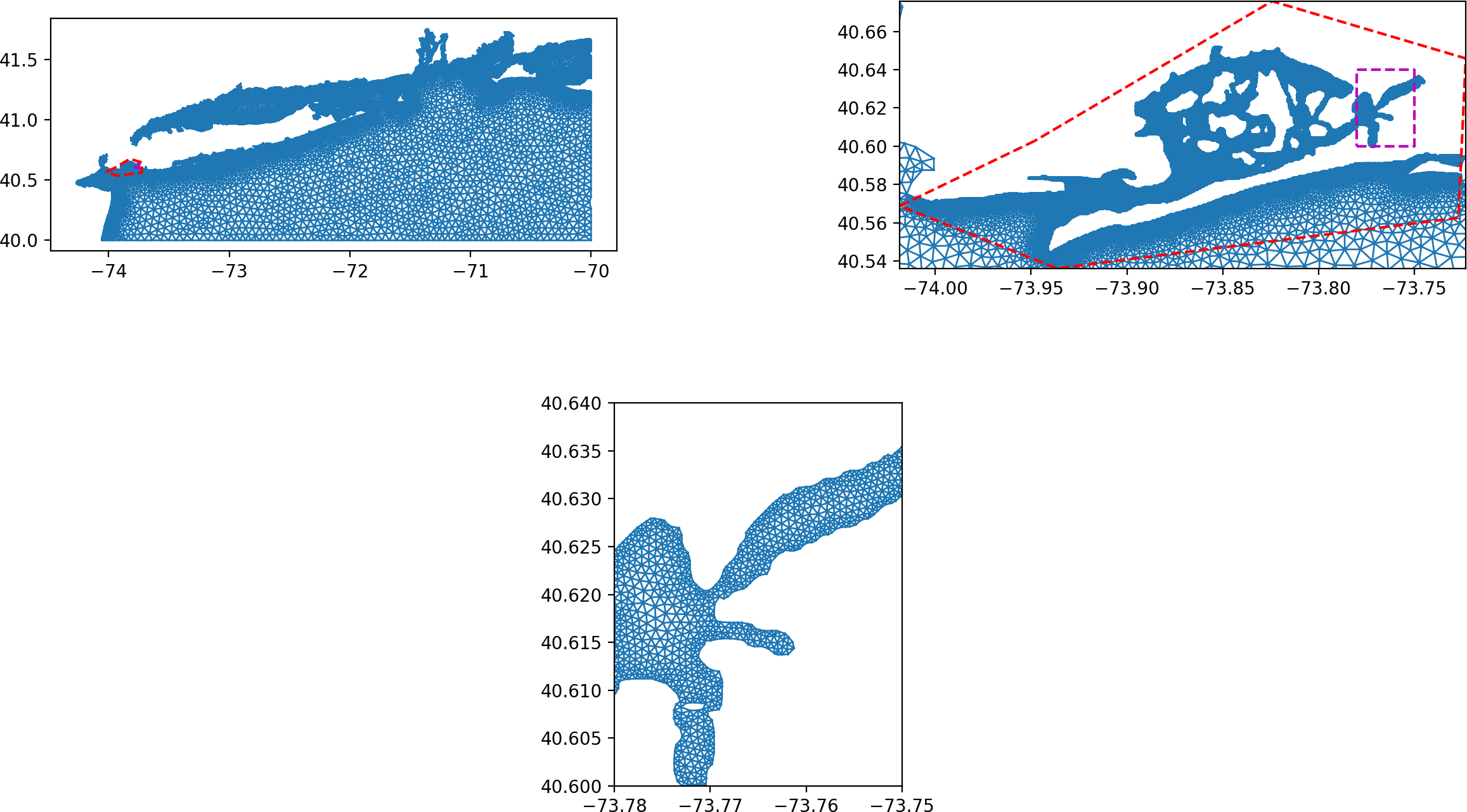
Multiscale mesh generation
The major downside of the DistMesh algorithm is that it cannot handle regional domains with fine mesh refinement or variable datasets due to the intense memory requirements. The multiscale mesh generation technique addresses these problems and enables an arbitrary number of refinement zones to be incorporated seamlessly into the domain.
Areas of finer refinement can be incorporated seamlessly by using the generate_multiscale_mesh function. In this case, the user passes lists of signed distance and edge length functions to the mesh generator but besides this the user API remains the same to the previous mesh generation example. The mesh sizing transitions between nests are handled automatically to produce meshes suitable for FEM and FVM numerical simulations through the parameters prefixed with "blend".
```python import matplotlib.gridspec as gridspec import matplotlib.pyplot as plt import matplotlib.tri as tri import numpy as np
import oceanmesh as om
fname = "gshhg-shp-2.3.7/GSHHSshp/f/GSHHSfL1.shp" EPSG = 4326 # EPSG:4326 or WGS84 extent1 = om.Region(extent=(-75.00, -70.001, 40.0001, 41.9000), crs=EPSG) minedgelength1 = 0.01 # minimum mesh size in domain in projection bbox2 = np.array( [ [-73.9481, 40.6028], [-74.0186, 40.5688], [-73.9366, 40.5362], [-73.7269, 40.5626], [-73.7231, 40.6459], [-73.8242, 40.6758], [-73.9481, 40.6028], ], dtype=float, ) extent2 = om.Region(extent=bbox2, crs=EPSG) minedgelength2 = 4.6e-4 # minimum mesh size in domain in projection s1 = om.Shoreline(fname, extent1.bbox, minedgelength1) sdf1 = om.signeddistancefunction(s1) el1 = om.distancesizingfunction(s1, maxedgelength=0.05) s2 = om.Shoreline(fname, extent2.bbox, minedgelength2) sdf2 = om.signeddistancefunction(s2) el2 = om.distancesizing_function(s2)
Control the element size transition
from coarse to fine with the kwargs prefixed with blend
points, cells = om.generatemultiscalemesh( [sdf1, sdf2], [el1, el2], )
remove degenerate mesh faces and other common problems in the mesh
points, cells = om.makemeshboundaries_traversable(points, cells)
remove singly connected elements (elements connected to only one other element)
points, cells = om.deletefacesconnectedtoone_face(points, cells)
remove poor boundary elements with quality < 15%
points, cells = om.deleteboundaryfaces(points, cells, min_qual=0.15)
apply a Laplacian smoother that preservers the mesh size distribution
points, cells = om.laplacian2(points, cells)
plot it showing the different levels of resolution
triang = tri.Triangulation(points[:, 0], points[:, 1], cells) gs = gridspec.GridSpec(2, 2) gs.update(wspace=0.5) plt.figure()
bbox3 = np.array( [ [-73.78, 40.60], [-73.75, 40.60], [-73.75, 40.64], [-73.78, 40.64], [-73.78, 40.60], ], dtype=float, )
ax = plt.subplot(gs[0, 0]) # ax.set_aspect("equal") ax.triplot(triang, "-", lw=1) ax.plot(bbox2[:, 0], bbox2[:, 1], "r--") ax.plot(bbox3[:, 0], bbox3[:, 1], "m--")
ax = plt.subplot(gs[0, 1]) ax.setaspect("equal") ax.triplot(triang, "-", lw=1) ax.plot(bbox2[:, 0], bbox2[:, 1], "r--") ax.setxlim(np.amin(bbox2[:, 0]), np.amax(bbox2[:, 0])) ax.set_ylim(np.amin(bbox2[:, 1]), np.amax(bbox2[:, 1])) ax.plot(bbox3[:, 0], bbox3[:, 1], "m--")
ax = plt.subplot(gs[1, :])
ax.setaspect("equal")
ax.triplot(triang, "-", lw=1)
ax.setxlim(-73.78, -73.75)
ax.set_ylim(40.60, 40.64)
plt.show()
```
Global mesh generation
Using oceanmesh is now possible for global meshes. The process is done in two steps: * first the definition of the sizing functions in WGS84 coordinates, * then the mesh generation is done in the stereographic projection
```python import os import numpy as np import oceanmesh as om from oceanmesh.region import tolatlon import matplotlib.pyplot as plt
utilities functions for plotting
def crosses_dateline(lon1, lon2): return abs(lon1 - lon2) > 180
def filtertriangles(points, cells): filteredcells = [] for cell in cells: p1, p2, p3 = points[cell[0]], points[cell[1]], points[cell[2]] if not (crossesdateline(p1[0], p2[0]) or crossesdateline(p2[0], p3[0]) or crossesdateline(p3[0], p1[0])): filteredcells.append(cell) return filtered_cells
Note: globalstereo.shp has been generated using globaltag() function in pyposeidon
https://github.com/ec-jrc/pyPoseidon/blob/9cfd3bbf5598c810004def83b1f43dc5149addd0/pyposeidon/boundary.py#L452
fname = "tests/global/globallatlon.shp" fname2 = "tests/global/globalstereo.shp"
EPSG = 4326 # EPSG:4326 or WGS84 bbox = (-180.00, 180.00, -89.00, 90.00) extent = om.Region(extent=bbox, crs=4326)
minedgelength = 0.5 # minimum mesh size in domain in meters maxedgelength = 2 # maximum mesh size in domain in meters shoreline = om.Shoreline(fname, extent.bbox, minedgelength) sdf = om.signeddistancefunction(shoreline) edgelength = om.distancesizing_function(shoreline, rate=0.11)
once the size functions have been defined, wed need to mesh inside domain in
stereographic projections. This is way we use another coastline which is
already translated in a sterographic projection
shorelinestereo = om.Shoreline(fname2, extent.bbox, minedgelength, stereo=True) domain = om.signeddistancefunction(shorelinestereo)
points, cells = om.generatemesh(domain, edgelength, stereo=True, max_iter=100)
remove degenerate mesh faces and other common problems in the mesh
points, cells = om.makemeshboundariestraversable(points, cells) points, cells = om.deletefacesconnectedtooneface(points, cells)
apply a Laplacian smoother
points, cells = om.laplacian2(points, cells, maxiter=100) lon, lat = tolatlon(points[:, 0], points[:, 1]) trin = filtertriangles(np.array([lon,lat]).T, cells)
fig, ax, pc = edgelength.plot(holding = True, plotcolorbar=True, cbarlabel = "Resolution in °", cmap='magma')
ax.triplot(lon, lat, trin, color="w", linewidth=0.25)
plt.tight_layout()
plt.show()
```
See the tests inside the testing/ folder for more inspiration. Work is ongoing on this package.
Testing
To run the oceanmesh unit tests (and turn off plots), check out this repository and type tox. tox can be installed via pip.
License
This software is published under the GPLv3 license
Owner
- Name: oceanmesh
- Login: CHLNDDEV
- Kind: user
- Website: https://keithroberts.site
- Repositories: 2
- Profile: https://github.com/CHLNDDEV
Developing automatic mesh generation technology for modeling the coastal ocean and floodplain
GitHub Events
Total
- Create event: 1
- Release event: 1
- Issues event: 4
- Watch event: 12
- Issue comment event: 17
- Push event: 5
- Pull request review comment event: 5
- Pull request review event: 2
- Pull request event: 3
- Fork event: 4
Last Year
- Create event: 1
- Release event: 1
- Issues event: 4
- Watch event: 12
- Issue comment event: 17
- Push event: 5
- Pull request review comment event: 5
- Pull request review event: 2
- Pull request event: 3
- Fork event: 4
Committers
Last synced: 10 months ago
Top Committers
| Name | Commits | |
|---|---|---|
| Keith Roberts | k****r@u****r | 24 |
| CHLNDDEV | 4****V | 5 |
| Thomas Saillour | s****s@g****m | 3 |
| Joseph Elmes | 4****e | 2 |
| Alain Coat | 9****t | 2 |
| Stefan Zieger | 9****r | 2 |
| Don Zimmer | d****r@b****m | 1 |
| Caio Eadi Stringari | c****i@g****m | 1 |
Issues and Pull Requests
Last synced: 9 months ago
All Time
- Total issues: 34
- Total pull requests: 50
- Average time to close issues: 3 months
- Average time to close pull requests: about 1 month
- Total issue authors: 12
- Total pull request authors: 12
- Average comments per issue: 2.0
- Average comments per pull request: 3.08
- Merged pull requests: 36
- Bot issues: 0
- Bot pull requests: 0
Past Year
- Issues: 3
- Pull requests: 2
- Average time to close issues: N/A
- Average time to close pull requests: about 7 hours
- Issue authors: 3
- Pull request authors: 2
- Average comments per issue: 2.0
- Average comments per pull request: 2.5
- Merged pull requests: 1
- Bot issues: 0
- Bot pull requests: 0
Top Authors
Issue Authors
- krober10nd (17)
- ml14je (3)
- tomsail (3)
- SorooshMani-NOAA (2)
- shuoli-code (1)
- ghost (1)
- loctk (1)
- filippogiaroli (1)
- liesvyvall (1)
- firesinger82 (1)
- caiostringari (1)
- ChengJungHsu (1)
Pull Request Authors
- krober10nd (31)
- tomsail (7)
- alcoat (3)
- ml14je (3)
- jcharris (2)
- sgriffithjones (2)
- stefanzieger (2)
- tomas19 (2)
- dpzimmer (1)
- liesvyvall (1)
- CHLNDDEV (1)
- caiostringari (1)
Top Labels
Issue Labels
Pull Request Labels
Dependencies
- actions/checkout v2 composite
- actions/setup-python v1 composite
- wearerequired/lint-action master composite
- actions/checkout v2 composite
- actions/setup-python v2 composite
- codecov/codecov-action v1 composite