apyxl

The apyxl package (Another PYthon package for eXplainable Learning) is a simple wrapper around xgboost, hyperopt, and shap. It provides the user with the ability to build a performant regression or classification model and use the power of the SHAP analysis to gain a better understanding of the links the model builds between its inputs and outputs. With apyxl, processing categorical features, fitting the model using Bayesian hyperparameter search, and instantiating the associated SHAP explainer can all be accomplished in a single line of code, streamlining the entire process from data preparation to model explanation.

The core of this package lies in the classes XGBClassifierWrapper and XGBRegressorWrapper. However, apyxl is not limited to these, as they also feed into the TimeSeriesNormalizer class, which enables the calculation of complex time series trends in an unsupervised manner.

More broadly, apyxl shapes my thinking on the connections between explainable machine learning, econometrics (Difference-In-Differences, Regression Discontinuity Design, Panel Analysis), time series normalization, and A/B testing.

Current Features

• Easy wrappers for regression and classification: apyxl.XGBClassifierWrapper and apyxl.XGBClassifierWrapper
• Automatic One-Hot-Encoding for categorical variables
• Bayesian hyperparameter optimization using hyperopt
• Simple explainability visualizations using shap (beeswarm, decision, force, scatter)
• apyxl.TimeSeriesNormalizer, a class designed to normalize a time series using other time series and compute a normalized time trend. This normalized trend is a time series that captures all the behavior of the analyzed time series that cannot be explained by the other series. While the original concept was developed for Weather Normalization, it can be extended to various non-weather-related features

Planned Enhancements

• A/B test analysis capabilities
• Formalizing the links between the two latest concepts, and comparison with econometrics techniques, like difference-in-differences, panel analysis and regression discontinuity. I believe these methods are closely related, and perhaps variations of a more general approach

NEW: I have conducted a numerical experiment demonstrating that the confidence often placed in p-values in econometrics can be misguided. Flawed or biased experimental designs may still result in very low p-values, leading to incorrect conclusions about causality.

NEW: I have started comparing apyxl with the discussed econometrics methods, beginning with Regression Discontinuity Design, have a look on this notebook.

Installation

To install the package, you can use Pypi:

bash pip install apyxl

Or you can use conda-forge:

bash conda install -c conda-forge apyxl

bash mamba install apyxl

Documentation

Documentation can be found here.

Basic Usage

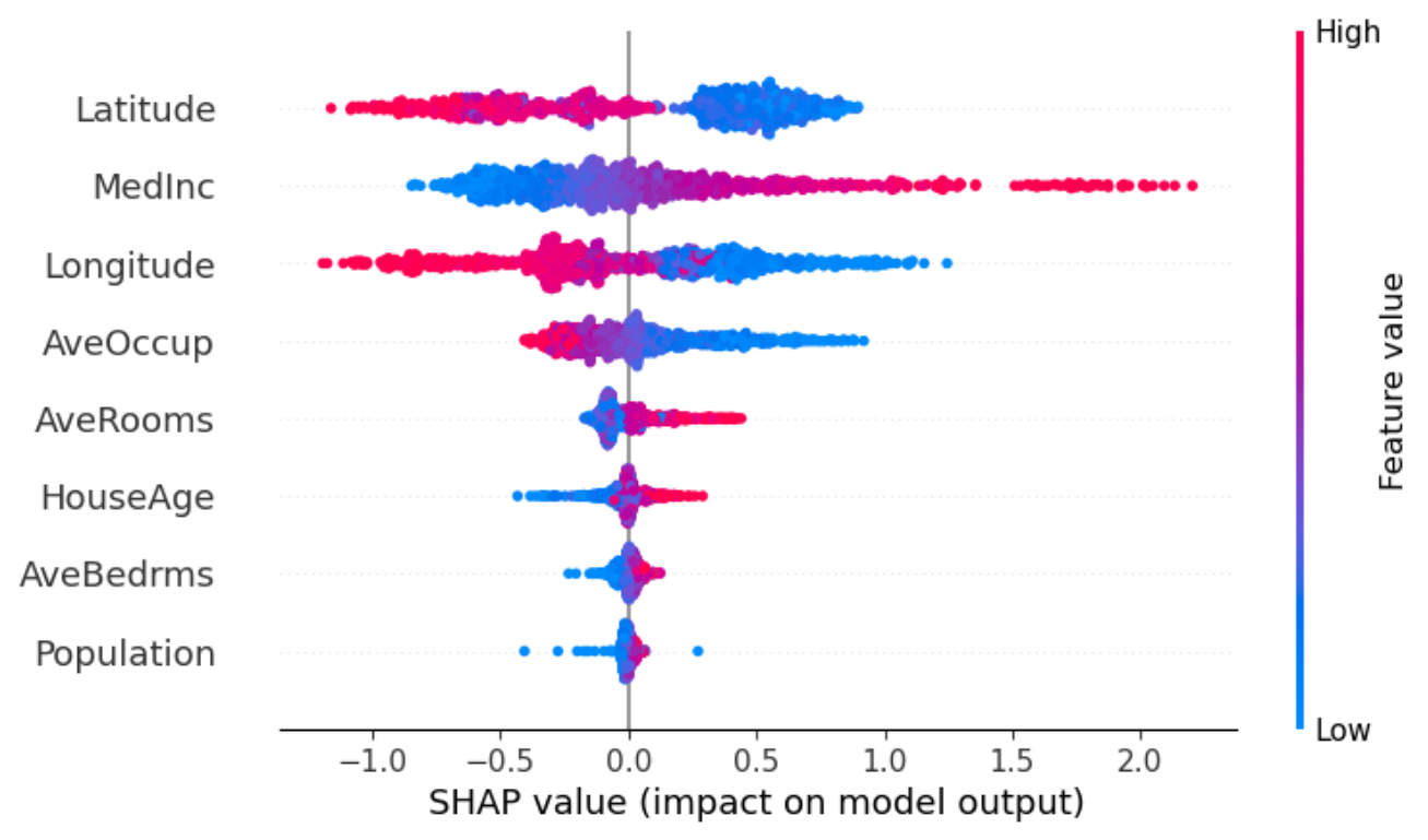
1. Regression

```python from apyxl import XGBRegressorWrapper from sklearn.datasets import fetchcaliforniahousing

X, y = fetchcaliforniahousing(asframe=True, returnX_y=True) X.shape, y.shape

((20640, 8), (20640,))

model = XGBRegressorWrapper().fit(X, y)

defaults to r2 score

model.best_score

0.6671771984999055

Plot methods can handle internally the computation of the SHAP values

model.beeswarm(X=X.sample(2_500)) ```

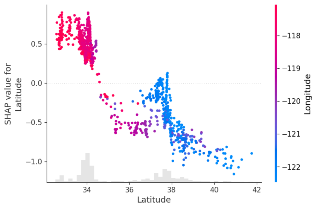
python model.scatter(X=X.sample(2_500), feature='Latitude')

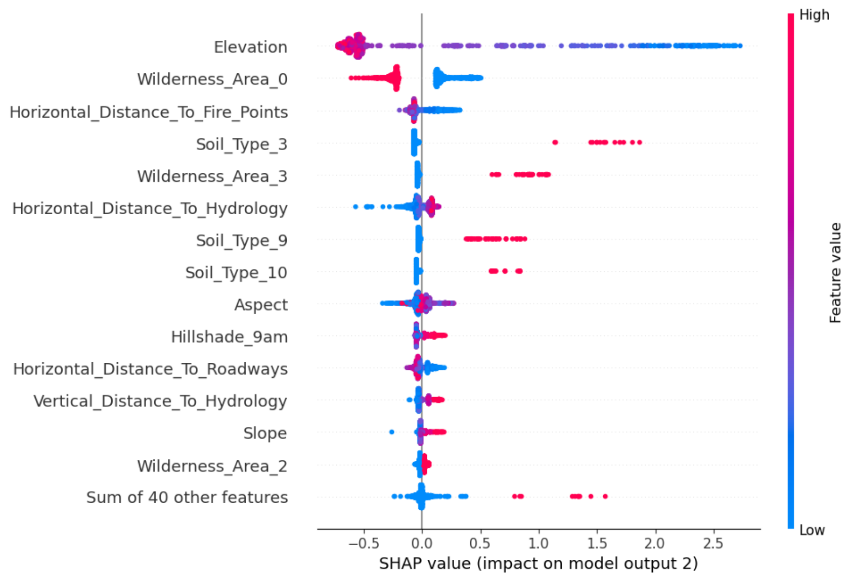
2. Classification

```python from apyxl import XGBClassifierWrapper from sklearn.datasets import fetch_covtype

X, y = fetchcovtype(asframe=True, returnXy=True) y -= 1 y.unique()

array([4, 1, 0, 6, 2, 5, 3])

X.shape, y.shape

((581012, 54), (581012,))

To speed up the process, Bayesian hyperparameter optimization can be performed on a subset of the

dataset. The model is then fitted on the entire dataset using the optimized hyperparameters.

model = XGBClassifierWrapper().fit(X, y, n=25_000)

defaults to Matthews correlation coefficient

model.best_score

0.5892932365687379

Computing SHAP values can be resource-intensive, so it's advisable to calculate them once for

multiple future uses, especially in multiclass classification scenarios where the cost is even

higher compared to binary classification (shap values shape equals (nsamples, nfeatures, n_classes))

shapvalues = model.computeshapvalues(X.sample(1000)) shap_values.shape

(1000, 54, 7)

The output argument selects the shap values associated to the desired class

model.beeswarm(shapvalues=shapvalues, output=2, max_display=15) ```

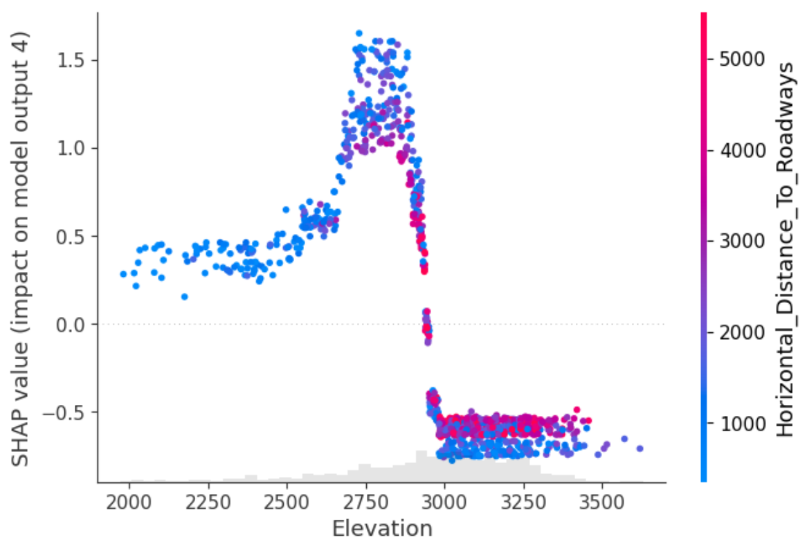
python model.scatter(shap_values=shap_values, feature='Elevation', output=4)

3. Time Series Normalization - A/B tests

3.1. Time Series Normalization

Weather normalization for time series is a trend discovery analysis that has long been used in weather-dependent applications (such as energy consumption or air pollution). My research suggests that it is equivalent to a SHAP analysis, treating time as a simple numeric variable. Tree-based methods like gradient boosting are particularly well-suited for discovering breakpoint changes, as they recursively split the dataset along one variable and one threshold.

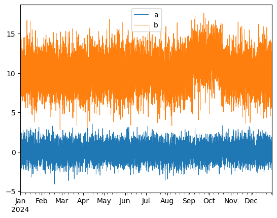
```python import matplotlib.pyplot as plt import numpy as np import pandas as pd from apyxl import XGBRegressorWrapper

n = 8760 time = pd.date_range(start='2024-01-01', freq='h', periods=n)

Generate two correlated time series, a and b

cov = [[1, 0.7], [0.7, 1]] mean = [0, 5]

df = np.random.multivariate_normal(cov=cov, mean=mean, size=n) df[:, 1] *= 2

Shift time serie b on a continuous subset of the period

df[6000:7000, 1] += 2

df = pd.DataFrame(df, columns=['a', 'b'], index=time)

df.plot(lw=0.7) plt.show() ```

```python

process time index as a simple numeric variable, i.e. the number of

days since the beginning of the dataset (could have been another time unit)

df['time_numeric'] = ((df.index - df.index.min())/pd.Timedelta(days=1)).astype(int)

apyxl can be then used as:

target = 'b' X, y = df.drop(columns=target), df[target] model = XGBRegressorWrapper(randomstate=0).fit(X, y) model.scatter(X, feature='a') model.scatter(X, feature='timenumeric') ```

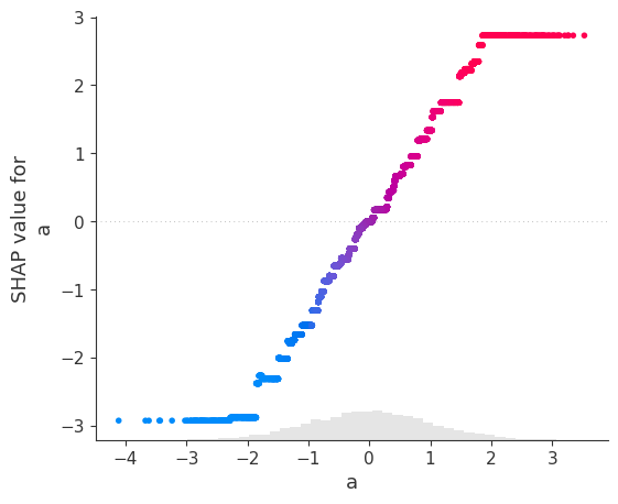
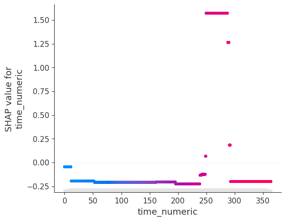
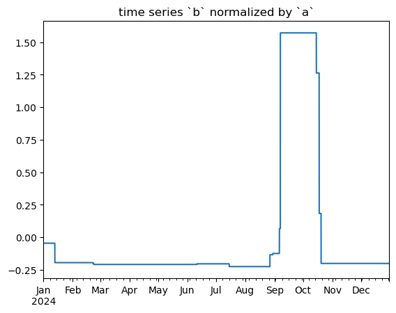
The fitted XGBoost regressor manages to capture the linear relationship between a and b (with the exception of extreme values) as well as the temporary, time-localized shift between the two time series. This trend, in other words the behavior of b that can't be explained by a, can be isolated:

python shap_values = model.compute_shap_values(X) pd.Series(shap_values[:, 'time_numeric'].values, index=X.index).plot(title='time series `b` normalized by `a`') plt.show()

All the previous can be condensed using apyxl.TimeSeriesNormalizer:

```python from apyxl import TimeSeriesNormalizer

tsn = TimeSeriesNormalizer(freq_trend='1d') trend = tsn.normalize(X=df, target='b') ```

3.2. A/B tests

Let's now look at our dataset in a different way: ```python import matplotlib.pyplot as plt import numpy as np import pandas as pd from apyxl import XGBRegressorWrapper

n = 8760 time = pd.date_range(start='2024-01-01', freq='h', periods=n)

Generate two correlated time series, a and b

cov = [[1, 0.7], [0.7, 1]] mean = [0, 5]

df = np.random.multivariate_normal(cov=cov, mean=mean, size=n) df[:, 1] *= 2

Shift time serie b on a continuous subset of the period

df[6000:7000, 1] += 2

df = pd.DataFrame(df, columns=['a', 'b'], index=time).renameaxis(index='time', columns='id') df = df.stack().rename('value').resetindex().setindex('time') df['timenumeric'] = ((df.index-df.index.min())/pd.Timedelta(days=1)).astype(int) df.sample(5)

                id     value  time_numeric

time
2024-12-24 05:00:00 a 1.944142 358 2024-09-01 11:00:00 a -0.528874 244 2024-10-26 22:00:00 b 7.377142 299 2024-04-17 03:00:00 a 0.744991 107 2024-12-15 11:00:00 b 8.370796 349 ```

We are now dealing with less structured data, with a value of interest and two different ids. Does the behavior of value change over time differently according to the ids?

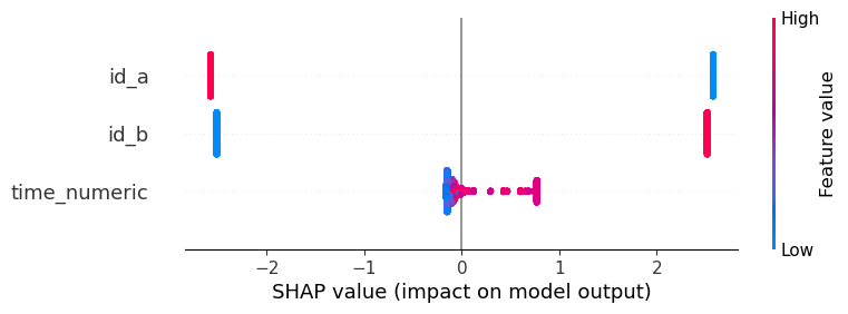
python target = 'value' X, y = df.drop(columns=target), df[target] model = XGBRegressorWrapper(max_evals=25).fit(X, y) model.beeswarm(X)

python model.scatter(X, feature='time_numeric')

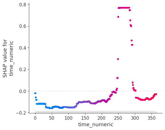
The SHAP analysis is clearly able to isolate relative changes of correlated time series over time.

The package's approach, using tree-based models like XGBoost for time series normalization and A/B testing, shares similarities with econometric techniques such as difference-in-differences (DiD) and fixed effects models. These methods aim to isolate the impact of treatments or events over time while controlling for confounding factors.

A key difference lies in the specification of events and variable impacts. In DiD, users must explicitly define event timing through dummy variables and quantify covariate effects through traditional econometric models. In contrast, this package's method can automatically discover relevant time periods without relying on prior user inputs and uses SHAP values to quantify variable impacts. This machine learning-based approach offers more flexibility by uncovering hidden events and interactions without explicit user-defined structures, while still providing interpretable results analogous to econometric models.

A future comparison between this approach and traditional econometric methods could yield valuable insights, particularly regarding non-linear relationships and the capture of complex interactions in time series data.

Note

Please note that this package is still under development, and features may change or expand in future versions.