<!-- -->

Blendpy is a computational toolkit for investigating thermodynamic models of alloys using first-principles calculations

Table of contents

• Installation
• Usage
  • Geometry optimization
  • Dilute solution interpolation (DSI) model
    • Enthalpy of mixing
    • DSI model from pre-calculated data
    • Polymorphism <!-- - Pseudo binary alloy -->
    • Ternary alloy
    • Phase diagram <!-- - Cluster expansion --> <!-- - Special quasirandom structure (SQS) --> <!-- - Intermetallics -->
• License
• Acknowledgements
• References

Installation

Install blendpy effortlessly using pip, Python’s default package manager, by running the following command in your terminal: sh pip install --upgrade pip pip install blendpy

Usage

This comprehensive tutorial guides you through calculating alloy properties. In this section, you'll learn how to determine key parameters—such as the enthalpy of mixing, and the spinodal and binodal decomposition curves derived from phase diagrams. We start by defining the alloy components, move through geometry optimization, and conclude with advanced modeling techniques using the DSI model.

To start, provide a list of structure files (e.g., CIF or POSCAR) that represent your alloy components. For best accuracy, it is recommended that these files have been pre-optimized using the same calculator and parameters that will be used in the subsequent alloy property calculations.

If you already have these optimized structures, you may skip ahead to the "DSI model" section. If not, proceed to the "Geometry Optimization" section to prepare your structures for analysis.

Geometry optimization

For example, let's calculate the properties of an Au-Pt alloy. We begin by retrieving the Au (fcc) and Pt (fcc) geometries from ASE. Next, we optimize these geometries using the MACE calculator, which leverages machine learning interatomic potentials.[^fn1] Finally, we save the optimized structures for use in the DSI model. To achieve this, we will follow several key steps.

Step 1: Import the necessary modules from ASE and MACE: python from ase.io import write from ase.build import bulk from ase.optimize import BFGSLineSearch from ase.filters import UnitCellFilter from mace.calculators import mace_mp

Step 2: Create Atoms objects for gold (Au) and platinum (Pt) using the bulk function: ```python

Create Au and Pt Atoms object

gold = bulk("Au", cubic=True) platinum = bulk("Pt", cubic=True) ```

Step 3: Create a MACE calculator object to optimize the structures and assign the calculator to the Atoms objects: ```python calcmace = macemp(model="small", dispersion=False, default_dtype="float32", device='cpu')

Assign the calculator to the Atoms objects

gold.calc = calcmace platinum.calc = calcmace ```

Step 4: Optimize the unit cells of Au and Pt using the BFGSLineSearch optimizer: ```python

Optimize Au and Pt unit cells

optimizergold = BFGSLineSearch(UnitCellFilter(gold)) optimizergold.run(fmax=0.01)

optimizerplatinum = BFGSLineSearch(UnitCellFilter(platinum)) optimizerplatinum.run(fmax=0.01) ```

Step 5: Save the optimized unit cells to CIF files: ```python

Save the optimized unit cells for Au and Pt

write("Aurelaxed.cif", gold) write("Ptrelaxed.cif", platinum) ```

Dilute solution interpolation (DSI) model

Enthalpy of mixing

Import the DSIModel from blendpy and create a DSIModel object using the optimized structures: ```python from blendpy import DSIModel

Create a DSIModel object

dsimodel = DSIModel(alloycomponents = ['Aurelaxed.cif', 'Ptrelaxed.cif'], supercell = [2,2,2], calculator = calc_mace) ```

Optimize the structures within the DSIModel object: ```python

Optimize the structures

dsi_model.optimize(method=BFGSLineSearch, fmax=0.01, logfile=None) ```

Calculate the enthalpy of mixing for the AuPt alloy: ```python

Calculate the enthalpy of mixing

enthalpyofmixing = dsimodel.getenthalpyofmixing(npoints=101) x = np.linspace(0, 1, len(enthalpyofmixing)) dfenthalpy = pd.DataFrame({'x': x, 'enthalpy': enthalpyof_mixing}) ```

Plotting the enthalpy of mixing ```python import numpy as np import matplotlib.pyplot as plt

fig, ax = plt.subplots(1,1, figsize=(5,5))

ax.setxlabel("$x$", fontsize=20) ax.setylabel("$\Delta H{mix}$ (kJ/mol)", fontsize=20) ax.setxlim(0,1) ax.setylim(-7,7) ax.setxticks(np.linspace(0,1,6)) ax.set_yticks(np.arange(-6,7,2))

Plot the data

color1='#fc4e2a' ax.plot(dfenthalpy['x'][::5], dfenthalpy['enthalpy'][::5], marker='o', color=color1, markersize=8, linewidth=3, zorder=2, label="DSI Model (MACE)")

REFERENCE: Okamoto, H. and Massalski, T., The Au-Pt (gold-platinum) system, Bull. Alloy Phase Diagr. 6, 46-56 (1985).

dfexp = pd.readcsv("data/experimental/expAuPt.csv") ax.plot(dfexp['x'], df_exp['enthalpy'], 's', color='grey', markersize=8, label="Exp. Data", zorder=1) ax.legend(loc="best", fontsize=16)

ax.tickparams(direction='in', axis='both', which='major', labelsize=20, width=3, length=8) ax.setboxaspect(1) for spine in ax.spines.values(): spine.setlinewidth(3)

plt.tight_layout()

plt.savefig("enthalpyofmixing.png", dpi=600, format='png', bbox_inches='tight')

plt.show() ```

Figure 1 - Enthalpy of mixing of the Au-Pt alloy computed using the DSI model and MACE interatomic potentials.

DSI model from pre-calculated data

Using blendpy, we can also calculate the enthalpy of mixing for an alloy based on DFT simulations that are not initiated by the DSIModel class object. Instead, we can use external data for the total energies of the pristine and dilute supercell systems. For instance, using the ab initio simulation software GPAW,[^fn2] we calculate the total energies for the Au-Pt alloy using [3,3,3] supercells of Au and Pt (Atoms(Au27) and Atoms(Pt27)), as well as the dilute systems (Atoms(Au26Pt) and Atoms(Pt26Au)). These total energies are then used to construct the energy matrix (energy_matrix) in the following form:

```python

energy_matrix = np.array([[ -85.940400, -89.230299], # [[ Au27, Au26Pt], [-170.278459, -173.891172]]) # [ Pt26Au, Pt27]] ```

Next, we demonstrate how to calculate the enthalpy of mixing using the input energy matrix.

```python import numpy as np import pandas as pd import matplotlib.pyplot as plt from ase.build import bulk from ase.io import write from blendpy import DSIModel

Create the two bulk structures

gold = bulk('Au', 'fcc') palladium = bulk('Pt', 'fcc')

Write the structures to CIF files

write("ciffiles/Au.cif", gold) write("ciffiles.Pt.cif", palladium)

Create the DSI model

alloycomponents = ['ciffiles/Au.cif', 'ciffiles/Pt.cif'] x0 = 1./27 dsimodel= DSIModel(alloycomponents=alloycomponents, supercell=[3,3,3], x0=x0)

Set the energy matrix

energy_matrix = np.array([[ -85.940400, -89.230299], [-170.278459, -173.891172]])

dsimodel.setenergymatrix(energymatrix)

enthalpy= dsimodel.getenthalpyofmixing()

x = np.linspace(0, 1, len(enthalpy))

df_enthalpy = pd.DataFrame({'x': x, 'enthalpy': enthalpy}) ```

In this case, it is MANDATORY to specify the minimum dilution factor (x0), the supercell size ([3,3,3]) used in the ab initio simulations, and the unit cell files ('Au.cif' and 'Pt.cif'). The unit cell files do not need to match exactly those used in the ab initio simulations.

Finally, we can plot the enthalpy of mixing and compare it with the experimental data.[^fn3] ```python

Plot the enthalpy of mixing

fig, ax = plt.subplots(1,1, figsize=(6,6))

ax.setxlabel('x', fontsize=20) ax.setylabel('$\Delta H{mix}$ (kJ/mol)', fontsize=20) ax.setxlim(0,1) ax.setylim(-7,7) ax.setxticks(np.linspace(0,1,6)) ax.setyticks(np.arange(-6,7,2)) ax.settitle("Au${1-x}$Pt${x}$", fontsize=20, pad=10)

plot data

Experimental

dfexp = pd.readcsv("../../data/experimental/expAuPt.csv") ax.plot(dfexp['x'], df_exp['enthalpy'], 's', color='grey', linestyle='--', linewidth=3, markersize=8, label="Exp. Data", zorder=1)

DSI model

ax.plot(dfenthalpy['x'][::5], dfenthalpy['enthalpy'][::5], marker='o', color='#fc4e2a', markersize=8, linewidth=3, zorder=2, label="DSI model from DFT")

ax.legend(fontsize=16, loc='best') ax.tickparams(axis='both', which='major', labelsize=20, width=3, length=8, direction='in') ax.setbox_aspect(1)

for spine in ax.spines.values(): spine.set_linewidth(3)

plt.tight_layout()

plt.savefig('enthalpyofmixingAuPtfrominput.png', dpi=400, bboxinches='tight')

plt.show() ```

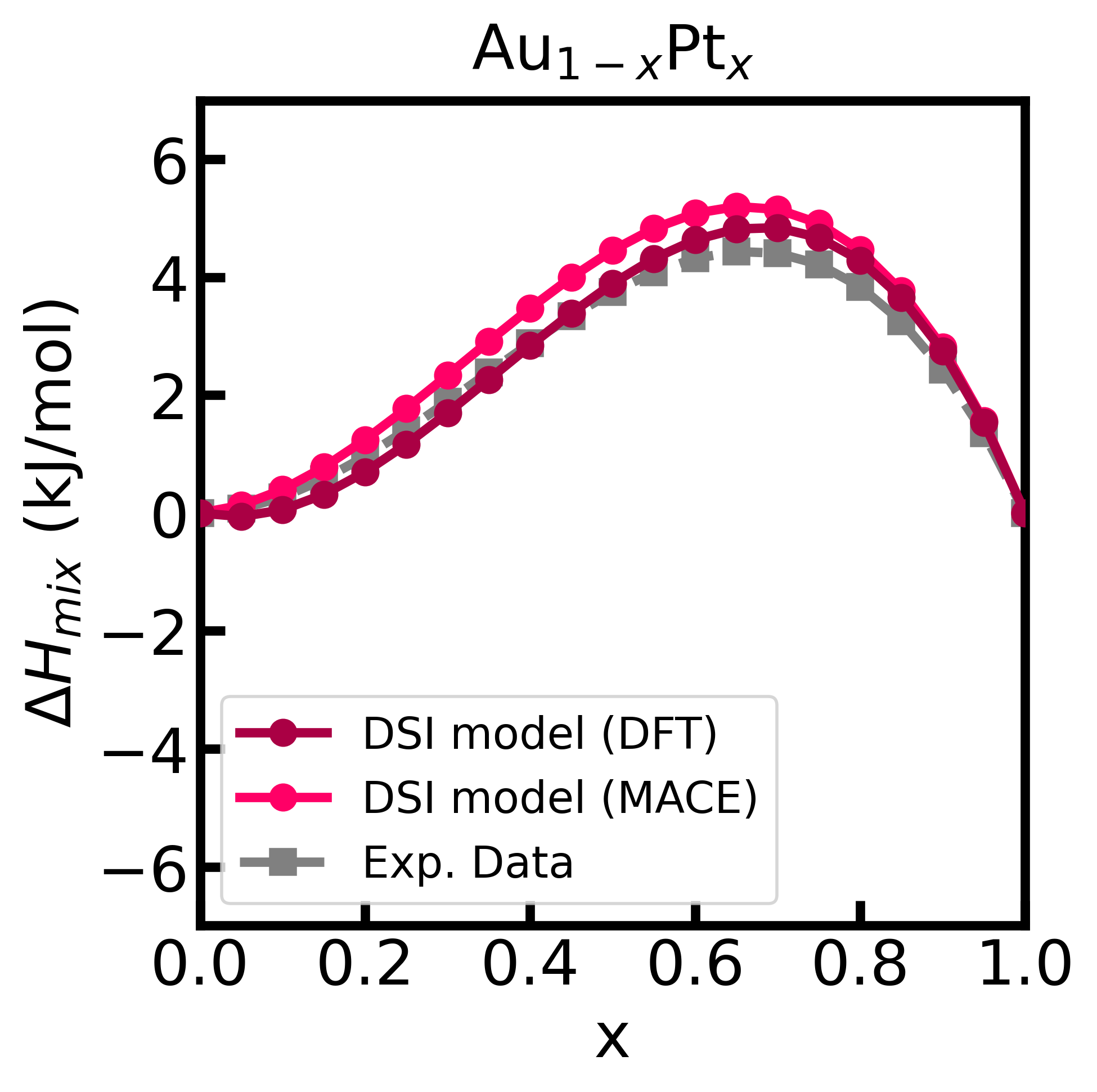
Figure 2 - Enthalpy of mixing of the Au-Pt alloy computed using the DSI model and energy matrix given from input (calculated with GPAW).

Polymorphism

Ternary alloy

Phase diagram (NOT WORKING)

By analyzing the mixing enthalpies and entropies, we can calculate the Gibbs free energy of the Au–Pt alloy mixture and determine both the spinodal and binodal (solvus) decomposition curves. These curves, which form key features of the alloy's phase diagram, delineate regions of differing stability: below the binodal curve, the solid solution (Au, Pt) is metastable, whereas it becomes unstable beneath the spinodal curve.

We begin by defining a temperature range over which to calculate the spinodal and binodal curves. Optionally, the results can be saved in CSV files. ```python

temperatures = np.arange(300, 3001, 5)

spinodal curve

dfspinodal = blendpy.getspinodaldecomposition(temperatures = temperatures, npoints = 501) dfspinodal.tocsv("data/phasediagram/spinodal_AuPt.csv", index=False, header=True, sep=',')

binodal curve

dfbinodal = blendpy.getbinodalcurve(temperatures = temperatures, npoints=501) dfbinodal.tocsv("data/phasediagram/binodal_AuPt.csv", index=False, header=True, sep=',') ```

To plot the phase diagram featuring the spinodal and binodal decomposition curves, we proceed as follows: ```python import pandas as pd

Create figure and axis

fig, ax = plt.subplots(1,1, figsize=(8,8))

x = np.linspace(0, 1, 101)

Configure axis labels and limits

ax.setxlabel("$x$", fontsize=20) ax.setylabel("$T$ (K)", fontsize=20) ax.setxlim(0,1) ax.setylim(300, 2500) ax.set_xticks(np.linspace(0,1,6))

Plot the data

ax.plot(dfspinodal['x'], dfspinodal['t'], color='#d53e4f', linestyle='--', linewidth=3, label="Spinodal curve") ax.plot(dfbinodal['x'], dfbinodal['t'], color='#d53e4f', linewidth=3, label="Binodal curve")

Fill below the curves with transparency (alpha=0.3 means 30% opacity)

ax.fillbetween(dfspinodal['x'], dfspinodal['t'], 300, color='#d53e4f', alpha=0.3) ax.fillbetween(dfbinodal['x'], dfbinodal['t'], 300, color='#d53e4f', alpha=0.3) ax.legend(loc="best", fontsize=20)

Add text annotations

ax.text(0.2, 1500, "Stable", fontsize=20, ha='center', va='center') ax.text(0.4, 950, "Metastable", fontsize=20, ha='center', va='center', rotation=60) ax.text(0.7, 700, "Unstable", fontsize=20, ha='center', va='center')

Customize tick parameters

ax.tickparams(direction='in', axis='both', which='major', labelsize=20, width=3, length=8) ax.setboxaspect(1) for spine in ax.spines.values(): spine.setlinewidth(3)

plt.tight_layout()

plt.savefig("phasediagram.png", dpi=600, format='png', bboxinches='tight')

plt.show() ```

Figure 2 - Phase diagram of the Au–Pt alloy computed using the DSI model and MACE interatomic potentials.

License

This is an open source code under MIT License.

Acknowledgements

We thank financial support from FAPESP (Grant No. 2022/14549-3), INCT Materials Informatics (Grant No. 406447/2022-5), and CNPq (Grant No. 311324/2020-7).

References

[^fn1]: Batatia, I., et al., MACE: Higher Order Equivariant Message Passing Neural Networks for Fast and Accurate Force Fields Adv. Neural Inf. Process Syst. 35, 11423 (2022).

[^fn2]: Mortensen, J. J., et al., GPAW: An open Python package for electronic structure calculations J. Chem. Phys. 160, 092503 (2024).

[^fn3]: Okamoto, H. and Massalski, T., The Au−Pt (Gold-Platinum) system Bull. Alloy Phase Diagr. 6, 46-56 (1985).