Science Score: 26.0%
This score indicates how likely this project is to be science-related based on various indicators:
-
○CITATION.cff file
-
✓codemeta.json file
Found codemeta.json file -
✓.zenodo.json file
Found .zenodo.json file -
○DOI references
-
○Academic publication links
-
○Committers with academic emails
-
○Institutional organization owner
-
○JOSS paper metadata
-
○Scientific vocabulary similarity
Low similarity (19.8%) to scientific vocabulary
Keywords from Contributors
geo
geofabrik-zone
osm-pbf
isochrones
opentripplanner
otp
public-transport
routing
transportation-planning
Last synced: 10 months ago
·
JSON representation
Repository
Get and reproduce data from the Propensity to Cycle Tool (PCT)
Basic Info
- Host: GitHub
- Owner: itsleeds
- Language: TeX
- Default Branch: master
- Homepage: https://itsleeds.github.io/pct/
- Size: 88.9 MB
Statistics
- Stars: 20
- Watchers: 5
- Forks: 10
- Open Issues: 3
- Releases: 11
Created over 7 years ago
· Last pushed over 1 year ago
Metadata Files
Readme
Changelog
README.Rmd
---
output: github_document
---
```{r setup, include = FALSE}
knitr::opts_chunk$set(
collapse = TRUE,
comment = "#>",
fig.path = "man/figures/README-",
out.width = "100%"
)
```
[](https://cran.r-project.org/package=pct)
[](https://github.com/itsleeds/pct/actions)
[](https://www.r-pkg.org/pkg/pct)
[](https://github.com/itsleeds/pct/actions/workflows/R-CMD-check.yaml)
# pct
The goal of pct is to make the data produced by the Propensity to Cycle Tool (PCT) easier to access and reproduce.
The PCT a research project and web application hosted at [www.pct.bike](https://www.pct.bike/).
For an overview of the data provided by the PCT, clicking on the previous link and trying it out is a great place to start.
An academic [paper](https://www.jtlu.org/index.php/jtlu/article/view/862) on the PCT provides detail on the motivations for and methods underlying the project.
A major motivation behind the project was making transport evidence more accessible, encouraging evidence-based transport policies.
The code base underlying the PCT is publicly available (see [github.com/npct](https://github.com/npct/)).
However, the code hosted there is not easy to run or reproduce, which is where this package comes in: it provides quick access to the data underlying the PCT and enables some of the key results to be reproduced quickly.
It was developed primarily for educational purposes (including for upcoming PCT training courses) but it may be useful for people to build on the the methods, for example to create a scenario of cycling uptake in their town/city/region.
In summary, if you want to know how PCT works, be able to reproduce some of its results, and build scenarios of cycling uptake to inform transport policies enabling cycling in cities worldwide, this package is for you!
## Installation
```{r, eval=FALSE}
# from CRAN
install.packages("pct")
```
You can install the development version of the package as follows:
```{r, eval=FALSE}
remotes::install_github("ITSLeeds/pct")
```
Load the package as follows:
```{r}
library(pct)
```
## Documentation
Probably the best place to get further information on the PCT is from the package's website at https://itsleeds.github.io/pct/
There you will find the following vignettes, which we recommend reading, and reproducing and experimenting with the code contained within to deepen your understanding of the code, in the following order:
1. A 'get started' introduction to the PCT and associated R package: https://itsleeds.github.io/pct/articles/pct.html
1. Getting and using PCT data, an [article](https://itsleeds.github.io/pct/articles/getting.html) showing how to get and use data from the PCT, based on a case study from North Yorkshire
1. A [training vignette](https://itsleeds.github.io/pct/articles/pct_training.html) providing more detailed guidance on data provided by the PCT package, with interactive exercises based on a case study of the Isle of Wight
1. A [vignette](https://itsleeds.github.io/pct/articles/cycling-potential-uk.html) show how to use the data provided by the package to estimate cycling uptake in UK cities
1. A [vignette](https://itsleeds.github.io/pct/articles/pct-international.html) demonstrating the international applicability of the PCT method, with help from this and other R packages
You will also find there documentation for each of the functions at [itsleeds.github.io/pct/reference/](https://itsleeds.github.io/pct/reference/index.html).
Below we describe some of the basics.
## Get PCT data
From feedback, we hear that the use of the data is critical in decision making. Therefore, one area where the package could be useful is making the data "easily" available to be processed.
* `get_pct`: the basic function to obtain data available [here](https://itsleeds.github.io/pct/reference/get_pct.html).
The rest of these should be self explanatory.
* `get_pct_centroids`
* `get_pct_lines`
* `get_pct_rnet`
* `get_pct_routes_fast`
* `get_pct_routes_quiet`
* `get_pct_zones`
* `uptake_pct_godutch`
* `uptake_pct_govtarget`
For example, to get the centroids in West Yorkshire:
``` {r centroids}
centroids = get_pct_centroids(region = "west-yorkshire")
plot(centroids[, "geo_name"])
```
Likewise to download the desire lines for "west-yorkshire":
```{r get_pct_lines}
lines = get_pct_lines(region = "west-yorkshire")
lines = lines[order(lines$all, decreasing = TRUE), c("all")]
plot(lines[1:10,], lwd = 4)
# view the lines on a map
# mapview::mapview(lines[1:3000, c("geo_name1")])
```
## Estimate cycling uptake
An important part of the PCT is its ability to create model scenarios of cycling uptake.
Key to the PCT uptake model is 'distance decay', meaning that short trips are more likely to be cycled than long trips.
The functions `uptake_pct_govtarget()` and `uptake_pct_godutch()` implement uptake models used in the PCT, which use distance and hilliness per desire line as inputs and output the proportion of people who could be expected to cycle if that scenario were realised.
The scenarios of cycling uptake produced by these functions are not predictions of what *will* happen, but illustrative snapshots of what *could* happen if overall propensity to cycle reached a certain level.
The uptake levels produced by Go Dutch and Government Target scenarios (which represent increases in cycling, not final levels) are illustrated in the graph below (other scenarios could be produced, see the [source code](https://itsleeds.github.io/pct/reference/uptake_pct_govtarget.html) see how these models work):
```{r decay}
max_distance = 50
distances = 1:max_distance
max_hilliness = 5
hilliness = 0:max_hilliness
uptake_df = data.frame(
distances = rep(distances, times = max_hilliness + 1),
hilliness = rep(hilliness, each = max_distance)
)
p_govtarget = uptake_pct_govtarget(
distance = uptake_df$distances,
gradient = uptake_df$hilliness
)
p_godutch = uptake_pct_godutch(
distance = uptake_df$distances,
gradient = uptake_df$hilliness
)
uptake_df = rbind(
cbind(uptake_df, scenario = "govtarget", pcycle = p_govtarget),
cbind(uptake_df, scenario = "godutch", pcycle = p_godutch)
)
library(ggplot2)
ggplot(uptake_df) +
geom_line(aes(
distances,
pcycle,
linetype = scenario,
colour = as.character(hilliness)
)) +
scale_color_discrete("Gradient (%)")
```
The proportion of trips made by cycling along each origin-destination (OD) pair therefore depends on the trip distance and hilliness.
The equivalent plot for hilliness is as follows:
```{r decayhills}
distances = c(1, 3, 6, 10, 15, 21)
hilliness = seq(0, 10, by = 0.2)
uptake_df =
data.frame(
expand.grid(distances, hilliness)
)
names(uptake_df) = c("distances", "hilliness")
p_govtarget = uptake_pct_govtarget(
distance = uptake_df$distances,
gradient = uptake_df$hilliness
)
p_godutch = uptake_pct_godutch(
distance = uptake_df$distances,
gradient = uptake_df$hilliness
)
uptake_df = rbind(
cbind(uptake_df, scenario = "govtarget", pcycle = p_govtarget),
cbind(uptake_df, scenario = "godutch", pcycle = p_godutch)
)
ggplot(uptake_df) +
geom_line(aes(
hilliness,
pcycle,
linetype = scenario,
colour = formatC(distances, flag = "0", width = 2)
)) +
scale_color_discrete("Distance (km)")
```
Note: if distances or gradient values appear to be provided in incorrect units, they will automatically be updated:
```{r}
distances = uptake_df$distances * 1000
hilliness = uptake_df$hilliness / 100
res = uptake_pct_godutch(distances, hilliness, verbose = TRUE)
```
The main input dataset into the PCT is OD data and, to convert each OD pair into a geographic desire line, geographic zone or centroids.
Typical input data is provided in packaged datasets `od_leeds` and `zones_leeds`, as shown in the next section.
## Reproduce PCT for Leeds
This example shows how scenarios of cycling uptake, and how 'distance decay' works (short trips are more likely to be cycled than long trips).
The input data looks like this (origin-destination data and geographic zone data):
```{r input-data}
class(od_leeds)
od_leeds[c(1:3, 12)]
class(zones_leeds)
zones_leeds[1:3, ]
```
The `stplanr` package can be used to convert the non-geographic OD data into geographic desire lines as follows:
```{r desire}
library(sf)
desire_lines = stplanr::od2line(flow = od_leeds, zones = zones_leeds[2])
plot(desire_lines[c(1:3, 12)])
```
We can convert these straight lines into routes with a routing service, e.g.:
```{r}
segments_fast = stplanr::route(l = desire_lines, route_fun = cyclestreets::journey)
```
We got useful information from this routing operation, we will convert the route segments into complete routes with `dplyr`:
```{r}
library(dplyr)
routes_fast = segments_fast %>%
group_by(area_of_residence, area_of_workplace) %>%
summarise(
all = unique(all),
bicycle = unique(bicycle),
length = sum(distances),
av_incline = mean(gradient_smooth) * 100
)
```
The results at the route level are as follows:
```{r routes_fast}
plot(routes_fast)
```
Now we estimate cycling uptake:
```{r}
routes_fast$uptake = uptake_pct_govtarget(distance = routes_fast$length, gradient = routes_fast$av_incline)
routes_fast$bicycle_govtarget = routes_fast$bicycle +
round(routes_fast$uptake * routes_fast$all)
```
Let's see how many people started cycling:
```{r}
sum(routes_fast$bicycle_govtarget) - sum(routes_fast$bicycle)
```
Nearly 1000 more people cycling to work, just in 10 desire is not bad!
What % cycling is this, for those routes?
```{r}
sum(routes_fast$bicycle_govtarget) / sum(routes_fast$all)
sum(routes_fast$bicycle) / sum(routes_fast$all)
```
It's gone from 4% to 11%, a realistic increase if cycling were enabled by good infrastructure and policies.
Now: where to prioritise that infrastructure and those policies?
```{r, eval=FALSE, echo=FALSE}
summary(sf::st_geometry_type(routes_fast))
```
```{r rnetgove, message=FALSE}
routes_fast_linestrings = sf::st_cast(routes_fast, "LINESTRING")
rnet = stplanr::overline(routes_fast_linestrings, attrib = c("bicycle", "bicycle_govtarget"))
lwd = rnet$bicycle_govtarget / mean(rnet$bicycle_govtarget)
plot(rnet["bicycle_govtarget"], lwd = lwd)
```
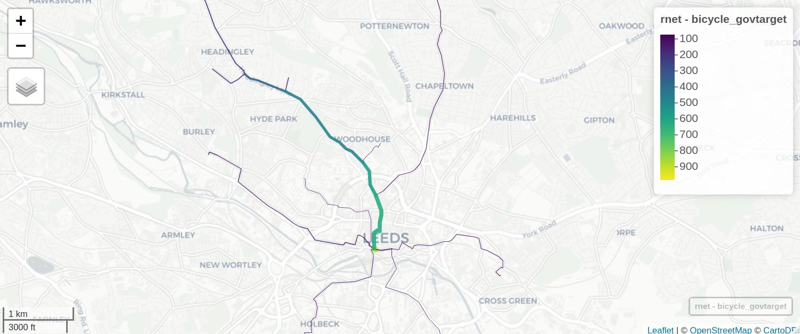
We can view the results in an interactive map and share with policy makers, stakeholders, and the public!
E.g. (see interactive map [here](https://rpubs.com/RobinLovelace/474074)):
```{r, eval=FALSE}
mapview::mapview(rnet, zcol = "bicycle_govtarget", lwd = lwd * 2)
```
## Limitations
* This package does not contain code to estimate cycling uptake associated with intrazonal flows and people with no fixed job data, although the datasets downloaded with the `get_pct_centroids()` functions provide estimated uptake for intrazonal flows.
* This package currently does not contiain code to estimate health benefits
## Testing the package
Test the package with the following code:
```{r, eval=FALSE}
remotes::install_github("ITSLeeds/pct")
devtools::check()
```
Owner
- Name: Institute for Transport Studies
- Login: ITSLeeds
- Kind: organization
- Location: Leeds, UK
- Website: https://environment.leeds.ac.uk/transport
- Repositories: 18
- Profile: https://github.com/ITSLeeds
GitHub Events
Total
- Watch event: 1
- Push event: 10
Last Year
- Watch event: 1
- Push event: 10
Committers
Last synced: 11 months ago
Top Committers
| Name | Commits | |
|---|---|---|
| Robin Lovelace | r****x@g****m | 410 |
| Layik Hama | l****a@g****m | 82 |
| joeytalbot | j****5@g****m | 17 |
| Nathanael Sheehan | n****n@g****m | 11 |
| Malcolm Morgan | m****8 | 3 |
| Haruko Nakao | 4****o | 2 |
| Dustin Carlino | d****r@g****m | 2 |
| Greta | 8****e | 1 |
Issues and Pull Requests
Last synced: 11 months ago
All Time
- Total issues: 84
- Total pull requests: 42
- Average time to close issues: 9 months
- Average time to close pull requests: 8 days
- Total issue authors: 13
- Total pull request authors: 8
- Average comments per issue: 4.11
- Average comments per pull request: 1.05
- Merged pull requests: 33
- Bot issues: 0
- Bot pull requests: 0
Past Year
- Issues: 0
- Pull requests: 0
- Average time to close issues: N/A
- Average time to close pull requests: N/A
- Issue authors: 0
- Pull request authors: 0
- Average comments per issue: 0
- Average comments per pull request: 0
- Merged pull requests: 0
- Bot issues: 0
- Bot pull requests: 0
Top Authors
Issue Authors
- Robinlovelace (64)
- layik (9)
- ccamara (1)
- temospena (1)
- edzer (1)
- Yuhei110 (1)
- Hussein-Mahfouz (1)
- ailishgraham (1)
- cristitosa (1)
- eugenividal (1)
- Whissi (1)
- mpadge (1)
- georgie5995 (1)
Pull Request Authors
- Robinlovelace (17)
- natesheehan (10)
- layik (5)
- joeytalbot (4)
- ccamara (2)
- HarukoNakao (2)
- GretaTimaite (1)
- dabreegster (1)
Top Labels
Issue Labels
good first issue (1)
enhancement (1)
Pull Request Labels
Packages
- Total packages: 3
-
Total downloads:
- cran 1,171 last-month
-
Total dependent packages: 4
(may contain duplicates) -
Total dependent repositories: 8
(may contain duplicates) - Total versions: 33
- Total maintainers: 1
proxy.golang.org: github.com/ITSLeeds/pct
- Documentation: https://pkg.go.dev/github.com/ITSLeeds/pct#section-documentation
-
Latest release: v0.9.9
published about 3 years ago
Rankings
Dependent packages count: 7.0%
Average: 8.2%
Dependent repos count: 9.3%
Last synced:
10 months ago
proxy.golang.org: github.com/itsleeds/pct
- Documentation: https://pkg.go.dev/github.com/itsleeds/pct#section-documentation
-
Latest release: v0.9.9
published about 3 years ago
Rankings
Dependent packages count: 7.0%
Average: 8.2%
Dependent repos count: 9.3%
Last synced:
10 months ago
cran.r-project.org: pct
Propensity to Cycle Tool
- Homepage: https://itsleeds.github.io/pct/
- Documentation: http://cran.r-project.org/web/packages/pct/pct.pdf
- License: GPL-3
-
Latest release: 0.10.0
published over 1 year ago
Rankings
Forks count: 6.9%
Dependent packages count: 9.1%
Dependent repos count: 10.6%
Average: 10.6%
Stargazers count: 12.2%
Downloads: 14.2%
Maintainers (1)
Last synced:
10 months ago
Dependencies
DESCRIPTION
cran
- R >= 3.5.0 depends
- boot * imports
- readr * imports
- sf * imports
- stplanr >= 0.2.8 imports
- bookdown * suggests
- covr * suggests
- curl * suggests
- dplyr * suggests
- ggplot2 * suggests
- knitr * suggests
- leaflet * suggests
- pbapply * suggests
- remotes * suggests
- rmarkdown * suggests
- testthat * suggests
- tidyverse * suggests
- tmap * suggests
.github/workflows/R-CMD-check.yaml
actions
- actions/cache v2 composite
- actions/checkout v2 composite
- actions/upload-artifact main composite
- r-lib/actions/setup-pandoc v1 composite
- r-lib/actions/setup-r v1 composite
.github/workflows/pkgdown.yaml
actions
- actions/cache v1 composite
- actions/checkout v2 composite
- r-lib/actions/setup-pandoc master composite
- r-lib/actions/setup-r master composite
.github/workflows/pr-commands.yaml
actions
- actions/checkout v2 composite
- r-lib/actions/pr-fetch master composite
- r-lib/actions/pr-push master composite
- r-lib/actions/setup-r master composite